Go to root: PhD-3D-Object-Tracking

It is time to learn the basics of one of the most interesting applications of point cloud processing: 3D object recognition. Akin to 2D recognition, this technique relies on finding good keypoints (characteristic points) in the cloud, and matching them to a set of previously saved ones. But 3D has several advantages over 2D: namely, we will be able to estimate with decent accuraccy the exact position and orientation of the object, relative to the sensor. Also, 3D object recognition tends to be more robust to clutter (crowded scenes where objects in the front occluding objects in the background). And finally, having information about the object's shape will help with collision avoidance or grasping operations.

In this first tutorial we will see what descriptors are, how many types are there available in PCL, and how to compute them.

Overview

The basis of 3D object recognition is to find a set of correspondences between two different clouds, one of them containing the object we are looking for. In order to do this, we need a way to compare points in an unambiguous manner. Until now, we have worked with points that store the XYZ coordinates, the RGB color... but none of those properties are unique enough. In two sequential scans, two points could share the same coordinates despite belonging to different surfaces, and using the color information takes us back to 2D recognition, will all the lightning related problems.

In a previous tutorial, we talked about features, before introducing the normals. Normals are an example of feature, because they encode information about the vicinity of the point. That is, the neighboring points are taken into account when computing it, giving us an idea of how the surrounding surface is. But this is not enough. For a feature to be optimal, it must meet the following criteria:

It must be robust to transformations: rigid transformations (the ones that do not change the distance between points) like translations and rotations must not affect the feature. Even if we play with the cloud a bit beforehand, there should be no difference.
It must be robust to noise: measurement errors that cause noise should not change the feature estimation much.
It must be resolution invariant: if sampled with different density (like after performing downsampling), the result must be identical or similar.

This is where descriptors come in. They are more complex (and precise) signatures of a point, that encode a lot of information about the surrounding geometry. The purpose is to unequivocally identify a point across multiple point clouds, no matter the noise, resolution or transformations. Also, some of them capture additional data about the object they belong to, like the viewpoint (that lets us retrieve the pose).

Finding correspondences between point features of two clouds (image from http://pointclouds.org/).

There are many 3D descriptors implemented into PCL. Each one has its own method for computing unique values for a point. Some use the difference between the angles of the normals of the point and its neighbors, for example. Others use the distances between the points. Because of this, some are inherently better or worse for certain purposes. A given descriptor may be scale invariant, and another one may be better with occlusions and partial views of objects. Which one you choose depends on what you want to do.

After calculating the necessary values, an additional step is performed to reduce the descriptor size: the result is binned into an histogram. To do this, the value range of each variable that makes up the descriptor is divided into n subdivisions, and the number of occurrences in each one is counted. Try to imagine a descriptor that computes a single variable, that ranges from 1 to 100. We choose to create 10 bins for it, so the first bin would gather all occurrences between 1 and 10, the second from 11 to 20, and so on. We look at the value of the variable for the first point-neighbor pair, and it is 27, so we increment the value of the third bin by 1. We keep doing this until we get a final histogram for that keypoint. The bin size must be carefully chosen depending on how descriptive that variable is (the variables do not have to share the same number of bins).

Descriptors can be classified in two main categories: global and local. The process for computing and using each one (recognition pipeline) is different, so each will be explained in its own section in this article.

Tutorials: How 3D Features work in PCL, Overview and Comparison of Features
Publication:
- Point Cloud Library: Three-Dimensional Object Recognition and 6 DoF Pose Estimation (Aitor Aldoma et al., 2012)

Local descriptors

Local descriptors are computed for individual points that we give as input. They have no notion of what an object is, they just describe how the local geometry is around that point. Usually, it is your task to choose which points you want a descriptor to be computed for: the keypoints. Most of the time, you can get away by just performing a downsampling and choosing all remaining points.

Local descriptors are used for object recognition and registration. Now we will see which ones are implemented into PCL.

PFH

PFH stands for Point Feature Histogram. It is one of the most important descriptors offered by PCL and the basis of others such as FPFH. The PFH tries to capture information of the geometry surrounding the point by analyzing the difference between the directions of the normals in the vicinity (and because of this, an imprecise normal estimation may produce low-quality descriptors).

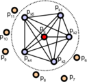
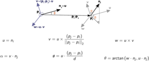
First, the algorithm pairs all points in the vicinity (not just the chosen keypoint with its neighbors, but also the neighbors with themselves). Then, for each pair, a fixed coordinate frame is computed from their normals. With this frame, the difference between the normals can be encoded with 3 angular variables. These variables, together with the euclidean distance between the points, are saved, and then binned to an histogram when all pairs have been computed. The final descriptor is the concatenation of the histograms of each variable (4 in total).

Point pairs established when computing the PFH for a point (image from http://pointclouds.org).
Fixed coordinate frame and angular features computed for one of the pairs (image from http://pointclouds.org).

Computing descriptors in PCL is very easy, and the PFH is not an exception:

#include <pcl/io/pcd_io.h>
#include <pcl/features/normal_3d.h>
#include <pcl/features/pfh.h>

int
main(int argc, char** argv)
{
	// Object for storing the point cloud.
	pcl::PointCloud<pcl::PointXYZ>::Ptr cloud(new pcl::PointCloud<pcl::PointXYZ>);
	// Object for storing the normals.
	pcl::PointCloud<pcl::Normal>::Ptr normals(new pcl::PointCloud<pcl::Normal>);
	// Object for storing the PFH descriptors for each point.
	pcl::PointCloud<pcl::PFHSignature125>::Ptr descriptors(new pcl::PointCloud<pcl::PFHSignature125> ());

	// Read a PCD file from disk.
	if (pcl::io::loadPCDFile<pcl::PointXYZ>(argv[1], *cloud) != 0)
	{
		return -1;
	}
	
	// Note: you would usually perform downsampling now. It has been omitted here
	// for simplicity, but be aware that computation can take a long time.

	// Estimate the normals.
	pcl::NormalEstimation<pcl::PointXYZ, pcl::Normal> normalEstimation;
	normalEstimation.setInputCloud(cloud);
	normalEstimation.setRadiusSearch(0.03);
	pcl::search::KdTree<pcl::PointXYZ>::Ptr kdtree(new pcl::search::KdTree<pcl::PointXYZ>);
	normalEstimation.setSearchMethod(kdtree);
	normalEstimation.compute(*normals);

	// PFH estimation object.
	pcl::PFHEstimation<pcl::PointXYZ, pcl::Normal, pcl::PFHSignature125> pfh;
	pfh.setInputCloud(cloud);
	pfh.setInputNormals(normals);
	pfh.setSearchMethod(kdtree);
	// Search radius, to look for neighbors. Note: the value given here has to be
	// larger than the radius used to estimate the normals.
	pfh.setRadiusSearch(0.05);

	pfh.compute(*descriptors);

	return 0;
}

As you can see, PCL uses the "PFHSignature125" type to save the descriptor to. This means that the descriptor's size is 125 (the dimensionality of the feature vector). Dividing a feature in D dimensional space in B divisions requires a total of B^D bins. The original proposal makes use of the distance between the points, but the implementation of PCL does not, as it was not considered discriminative enough (specially in 2.5D scans, where the distance between points increases the further away from the sensor). Hence, the remaining features (with one dimension each) can be divided in 5 divisions, resulting in a 125-dimensional (5³) vector.

The final object that stores the computed descriptors can be handled like a normal cloud (even saved to, or read from, disk), and it has the same number of "points" than the original one. The "PFHSignature125" object at position 0, for example, stores the PFH descriptor for the "PointXYZ" point at the same position in the cloud.

For additional details about the descriptor, check the original publications listed below, or PCL's tutorial.

Input: Points, Normals, Search method, Radius
Output: PFH descriptors
Tutorial: Point Feature Histograms (PFH) descriptors
Publications:
- Persistent Point Feature Histograms for 3D Point Clouds (Radu Bogdan Rusu et al., 2008)
- Semantic 3D Object Maps for Everyday Manipulation in Human Living Environments (Radu Bogdan Rusu, 2009, section 4.4, page 50)
API: pcl::PFHEstimation
Download

FPFH

PFH gives accurate results, but it has a drawback: it is too computationally expensive to perform at real time. For a cloud of n keypoints with k neighbors considered, it has a complexity of O(nk²). Because of this, a derived descriptor was created, named FPFH (Fast Point Feature Histogram).

The FPFH considers only the direct connections between the current keypoint and its neighbors, removing additional links between neighbors. This takes the complexity down to O(nk). Because of this, the resulting histogram is referred to as SPFH (Simplified Point Feature Histogram). The reference frame and the angular variables are computed as always.

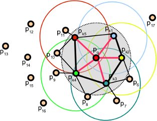
Point pairs established when computing the FPFH for a point (image from http://pointclouds.org).

To account for the loss of these extra connections, an additional step takes place after all histograms have been computed: the SPFHs of a point's neighbors are "merged" with its own, weighted according to the distance. This has the effect of giving a point surface information of points as far away as 2 times the radius used. Finally, the 3 histograms (distance is not used) are concatenated to compose the final descriptor.

#include <pcl/io/pcd_io.h>
#include <pcl/features/normal_3d.h>
#include <pcl/features/fpfh.h>

int
main(int argc, char** argv)
{
	// Object for storing the point cloud.
	pcl::PointCloud<pcl::PointXYZ>::Ptr cloud(new pcl::PointCloud<pcl::PointXYZ>);
	// Object for storing the normals.
	pcl::PointCloud<pcl::Normal>::Ptr normals(new pcl::PointCloud<pcl::Normal>);
	// Object for storing the FPFH descriptors for each point.
	pcl::PointCloud<pcl::FPFHSignature33>::Ptr descriptors(new pcl::PointCloud<pcl::FPFHSignature33> ());

	// Read a PCD file from disk.
	if (pcl::io::loadPCDFile<pcl::PointXYZ>(argv[1], *cloud) != 0)
	{
		return -1;
	}
	
	// Note: you would usually perform downsampling now. It has been omitted here
	// for simplicity, but be aware that computation can take a long time.

	// Estimate the normals.
	pcl::NormalEstimation<pcl::PointXYZ, pcl::Normal> normalEstimation;
	normalEstimation.setInputCloud(cloud);
	normalEstimation.setRadiusSearch(0.03);
	pcl::search::KdTree<pcl::PointXYZ>::Ptr kdtree(new pcl::search::KdTree<pcl::PointXYZ>);
	normalEstimation.setSearchMethod(kdtree);
	normalEstimation.compute(*normals);

	// FPFH estimation object.
	pcl::FPFHEstimation<pcl::PointXYZ, pcl::Normal, pcl::FPFHSignature33> fpfh;
	fpfh.setInputCloud(cloud);
	fpfh.setInputNormals(normals);
	fpfh.setSearchMethod(kdtree);
	// Search radius, to look for neighbors. Note: the value given here has to be
	// larger than the radius used to estimate the normals.
	fpfh.setRadiusSearch(0.05);

	fpfh.compute(*descriptors);

	return 0;
}

An additional implementation of the FPFH estimation that takes advantage of multithreaded optimizations (with the OpenMP API) is available in the class "FPFHEstimationOMP". Its interface is identical to the standard unoptimized implementation. Using it will result in a big performance boost on multi-core systems, meaning faster computation times. Remember to include the header "fpfh_omp.h" instead.

Input: Points, Normals, Search method, Radius
Output: FPFH descriptors
Tutorial: Fast Point Feature Histograms (FPFH) descriptors
Publications:
- Fast Point Feature Histograms (FPFH) for 3D Registration (Radu Bogdan Rusu et al., 2009)
- Semantic 3D Object Maps for Everyday Manipulation in Human Living Environments (Radu Bogdan Rusu, 2009, section 4.5, page 57)
API: pcl::FPFHEstimation, pcl::FPFHEstimationOMP
Download

RSD

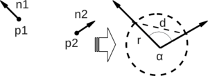
The Radius-Based Surface Descriptor encodes the radial relationship of the point and its neighborhood. For every pair of the keypoint with a neighbor, the algorithm computes the distance between them, and the difference between their normals. Then, by assuming that both points lie on the surface of a sphere, said sphere is found by fitting not only the points, but also the normals (otherwise, there would be infinite possible spheres). Finally, from all the point-neighbor spheres, only the ones with the maximum and minimum radii are kept and saved to the descriptor of that point.

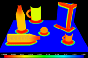
As you may have deduced already, when two points lie on a flat surface, the sphere radius will be infinite. If, on the other hand, they lie on the curved face of a cylinder, the radius will be more or less the same as that of the cylinder. This allows us to tell apart objects with RSD. The algorithm takes a parameter that sets the maximum radius at which the points will be considered to be part of a plane.

Sphere that fits two points with their normals (image from original presentation).
RSD values for a cloud; points on a flat surface have maximum values (image from original presentation).

Currently, the RSD estimator class is not available in PCL (the code has been commented out) because it lacked proper testing and documentation (for more details, see the issue or this post on the mailing list). When it is restored, I will provide a code snippet as always.

Input: Points, Normals, Search method, Radius, Maximum Radius
Output: RSD descriptors
Publication:
- General 3D Modelling of Novel Objects from a Single View (Zoltan-Csaba Marton et al., 2009)
API: pcl::RSDEstimation