PCL/OpenNI tutorial 4: 3D object recognition (descriptors)
Go to root: PhD-3D-Object-Tracking
It is time to learn the basics of one of the most interesting applications of point cloud processing: 3D object recognition. Akin to 2D recognition, this technique relies on finding good keypoints (characteristic points) in the cloud, and matching them to a set of previously saved ones. But 3D has several advantages over 2D: namely, we will be able to estimate with decent accuracy the exact position and orientation of the object, relative to the sensor. Also, 3D object recognition tends to be more robust to clutter (crowded scenes where objects in the front occluding objects in the background). And finally, having information about the object's shape will help with collision avoidance or grasping operations.
In this first tutorial we will see what descriptors are, how many types are there available in PCL, and how to compute them.
Overview
The basis of 3D object recognition is to find a set of correspondences between two different clouds, one of them containing the object we are looking for. In order to do this, we need a way to compare points in an unambiguous manner. Until now, we have worked with points that store the XYZ coordinates, the RGB color... but none of those properties are unique enough. In two sequential scans, two points could share the same coordinates despite belonging to different surfaces, and using the color information takes us back to 2D recognition, will all the lightning related problems.
In a previous tutorial, we talked about features, before introducing the normals. Normals are an example of feature, because they encode information about the vicinity of the point. That is, the neighboring points are taken into account when computing it, giving us an idea of how the surrounding surface is. But this is not enough. For a feature to be optimal, it must meet the following criteria:
- It must be robust to transformations: rigid transformations (the ones that do not change the distance between points) like translations and rotations must not affect the feature. Even if we play with the cloud a bit beforehand, there should be no difference.
- It must be robust to noise: measurement errors that cause noise should not change the feature estimation much.
- It must be resolution invariant: if sampled with different density (like after performing downsampling), the result must be identical or similar.
This is where descriptors come in. They are more complex (and precise) signatures of a point, that encode a lot of information about the surrounding geometry. The purpose is to unequivocally identify a point across multiple point clouds, no matter the noise, resolution or transformations. Also, some of them capture additional data about the object they belong to, like the viewpoint (that lets us retrieve the pose).

There are many 3D descriptors implemented into PCL. Each one has its own method for computing unique values for a point. Some use the difference between the angles of the normals of the point and its neighbors, for example. Others use the distances between the points. Because of this, some are inherently better or worse for certain purposes. A given descriptor may be scale invariant, and another one may be better with occlusions and partial views of objects. Which one you choose depends on what you want to do.
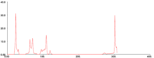
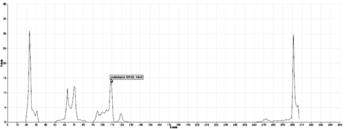
After calculating the necessary values, an additional step is performed to reduce the descriptor size: the result is binned into an histogram. To do this, the value range of each variable that makes up the descriptor is divided into n subdivisions, and the number of occurrences in each one is counted. Try to imagine a descriptor that computes a single variable, that ranges from 1 to 100. We choose to create 10 bins for it, so the first bin would gather all occurrences between 1 and 10, the second from 11 to 20, and so on. We look at the value of the variable for the first point-neighbor pair, and it is 27, so we increment the value of the third bin by 1. We keep doing this until we get a final histogram for that keypoint. The bin size must be carefully chosen depending on how descriptive that variable is (the variables do not have to share the same number of bins).
Descriptors can be classified in two main categories: global and local. The process for computing and using each one (recognition pipeline) is different, so each will be explained in its own section in this article.
- Tutorials: How 3D Features work in PCL, Overview and Comparison of Features
- Publication:
- Point Cloud Library: Three-Dimensional Object Recognition and 6 DoF Pose Estimation (Aitor Aldoma et al., 2012)
Local descriptors
Local descriptors are computed for individual points that we give as input. They have no notion of what an object is, they just describe how the local geometry is around that point. Usually, it is your task to choose which points you want a descriptor to be computed for: the keypoints. Most of the time, you can get away by just performing a downsampling and choosing all remaining points.
Local descriptors are used for object recognition and registration. Now we will see which ones are implemented into PCL.
PFH
PFH stands for Point Feature Histogram. It is one of the most important descriptors offered by PCL and the basis of others such as FPFH. The PFH tries to capture information of the geometry surrounding the point by analyzing the difference between the directions of the normals in the vicinity (and because of this, an imprecise normal estimation may produce low-quality descriptors).
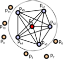
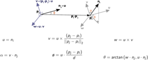
First, the algorithm pairs all points in the vicinity (not just the chosen keypoint with its neighbors, but also the neighbors with themselves). Then, for each pair, a fixed coordinate frame is computed from their normals. With this frame, the difference between the normals can be encoded with 3 angular variables. These variables, together with the euclidean distance between the points, are saved, and then binned to an histogram when all pairs have been computed. The final descriptor is the concatenation of the histograms of each variable (4 in total).
Point pairs established when computing the PFH for a point (image from http://pointclouds.org).
Fixed coordinate frame and angular features computed for one of the pairs (image from http://pointclouds.org).
Computing descriptors in PCL is very easy, and the PFH is not an exception:
#include <pcl/io/pcd_io.h>
#include <pcl/features/normal_3d.h>
#include <pcl/features/pfh.h>

int
main(int argc, char** argv)
{
	// Object for storing the point cloud.
	pcl::PointCloud<pcl::PointXYZ>::Ptr cloud(new pcl::PointCloud<pcl::PointXYZ>);
	// Object for storing the normals.
	pcl::PointCloud<pcl::Normal>::Ptr normals(new pcl::PointCloud<pcl::Normal>);
	// Object for storing the PFH descriptors for each point.
	pcl::PointCloud<pcl::PFHSignature125>::Ptr descriptors(new pcl::PointCloud<pcl::PFHSignature125>());

	// Read a PCD file from disk.
	if (pcl::io::loadPCDFile<pcl::PointXYZ>(argv[1], *cloud) != 0)
	{
		return -1;
	}

	// Note: you would usually perform downsampling now. It has been omitted here
	// for simplicity, but be aware that computation can take a long time.

	// Estimate the normals.
	pcl::NormalEstimation<pcl::PointXYZ, pcl::Normal> normalEstimation;
	normalEstimation.setInputCloud(cloud);
	normalEstimation.setRadiusSearch(0.03);
	pcl::search::KdTree<pcl::PointXYZ>::Ptr kdtree(new pcl::search::KdTree<pcl::PointXYZ>);
	normalEstimation.setSearchMethod(kdtree);
	normalEstimation.compute(*normals);

	// PFH estimation object.
	pcl::PFHEstimation<pcl::PointXYZ, pcl::Normal, pcl::PFHSignature125> pfh;
	pfh.setInputCloud(cloud);
	pfh.setInputNormals(normals);
	pfh.setSearchMethod(kdtree);
	// Search radius, to look for neighbors. Note: the value given here has to be
	// larger than the radius used to estimate the normals.
	pfh.setRadiusSearch(0.05);

	pfh.compute(*descriptors);
}
As you can see, PCL uses the "PFHSignature125" type to save the descriptor to. This means that the descriptor's size is 125 (the dimensionality of the feature vector). Dividing a feature in D dimensional space in B divisions requires a total of BD bins. The original proposal makes use of the distance between the points, but the implementation of PCL does not, as it was not considered discriminative enough (specially in 2.5D scans, where the distance between points increases the further away from the sensor). Hence, the remaining features (with one dimension each) can be divided in 5 divisions, resulting in a 125-dimensional (53) vector.
The final object that stores the computed descriptors can be handled like a normal cloud (even saved to, or read from, disk), and it has the same number of "points" than the original one. The "PFHSignature125" object at position 0, for example, stores the PFH descriptor for the "PointXYZ" point at the same position in the cloud.
For additional details about the descriptor, check the original publications listed below, or PCL's tutorial.
- Input: Points, Normals, Search method, Radius
- Output: PFH descriptors
- Tutorial: Point Feature Histograms (PFH) descriptors
- Publications:
- Persistent Point Feature Histograms for 3D Point Clouds (Radu Bogdan Rusu et al., 2008)
- Semantic 3D Object Maps for Everyday Manipulation in Human Living Environments (Radu Bogdan Rusu, 2009, section 4.4, page 50)
- API: pcl::PFHEstimation
- Download
FPFH
PFH gives accurate results, but it has a drawback: it is too computationally expensive to perform at real time. For a cloud of n keypoints with k neighbors considered, it has a complexity of O(nk2). Because of this, a derived descriptor was created, named FPFH (Fast Point Feature Histogram).
The FPFH considers only the direct connections between the current keypoint and its neighbors, removing additional links between neighbors. This takes the complexity down to O(nk). Because of this, the resulting histogram is referred to as SPFH (Simplified Point Feature Histogram). The reference frame and the angular variables are computed as always.
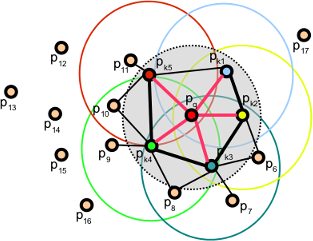
To account for the loss of these extra connections, an additional step takes place after all histograms have been computed: the SPFHs of a point's neighbors are "merged" with its own, weighted according to the distance. This has the effect of giving a point surface information of points as far away as 2 times the radius used. Finally, the 3 histograms (distance is not used) are concatenated to compose the final descriptor.
#include <pcl/io/pcd_io.h>
#include <pcl/features/normal_3d.h>
#include <pcl/features/fpfh.h>

int
main(int argc, char** argv)
{
	// Object for storing the point cloud.
	pcl::PointCloud<pcl::PointXYZ>::Ptr cloud(new pcl::PointCloud<pcl::PointXYZ>);
	// Object for storing the normals.
	pcl::PointCloud<pcl::Normal>::Ptr normals(new pcl::PointCloud<pcl::Normal>);
	// Object for storing the FPFH descriptors for each point.
	pcl::PointCloud<pcl::FPFHSignature33>::Ptr descriptors(new pcl::PointCloud<pcl::FPFHSignature33>());

	// Read a PCD file from disk.
	if (pcl::io::loadPCDFile<pcl::PointXYZ>(argv[1], *cloud) != 0)
	{
		return -1;
	}

	// Note: you would usually perform downsampling now. It has been omitted here
	// for simplicity, but be aware that computation can take a long time.

	// Estimate the normals.
	pcl::NormalEstimation<pcl::PointXYZ, pcl::Normal> normalEstimation;
	normalEstimation.setInputCloud(cloud);
	normalEstimation.setRadiusSearch(0.03);
	pcl::search::KdTree<pcl::PointXYZ>::Ptr kdtree(new pcl::search::KdTree<pcl::PointXYZ>);
	normalEstimation.setSearchMethod(kdtree);
	normalEstimation.compute(*normals);

	// FPFH estimation object.
	pcl::FPFHEstimation<pcl::PointXYZ, pcl::Normal, pcl::FPFHSignature33> fpfh;
	fpfh.setInputCloud(cloud);
	fpfh.setInputNormals(normals);
	fpfh.setSearchMethod(kdtree);
	// Search radius, to look for neighbors. Note: the value given here has to be
	// larger than the radius used to estimate the normals.
	fpfh.setRadiusSearch(0.05);

	fpfh.compute(*descriptors);
}
An additional implementation of the FPFH estimation that takes advantage of multithreaded optimizations (with the OpenMP API) is available in the class "FPFHEstimationOMP". Its interface is identical to the standard unoptimized implementation. Using it will result in a big performance boost on multi-core systems, meaning faster computation times. Remember to include the header "fpfh_omp.h" instead.
- Input: Points, Normals, Search method, Radius
- Output: FPFH descriptors
- Tutorial: Fast Point Feature Histograms (FPFH) descriptors
- Publications:
- Fast Point Feature Histograms (FPFH) for 3D Registration (Radu Bogdan Rusu et al., 2009)
- Semantic 3D Object Maps for Everyday Manipulation in Human Living Environments (Radu Bogdan Rusu, 2009, section 4.5, page 57)
- API: pcl::FPFHEstimation, pcl::FPFHEstimationOMP
- Download
RSD
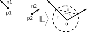
The Radius-Based Surface Descriptor encodes the radial relationship of the point and its neighborhood. For every pair of the keypoint with a neighbor, the algorithm computes the distance between them, and the difference between their normals. Then, by assuming that both points lie on the surface of a sphere, said sphere is found by fitting not only the points, but also the normals (otherwise, there would be infinite possible spheres). Finally, from all the point-neighbor spheres, only the ones with the maximum and minimum radii are kept and saved to the descriptor of that point.
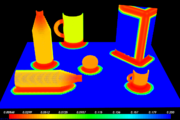
As you may have deduced already, when two points lie on a flat surface, the sphere radius will be infinite. If, on the other hand, they lie on the curved face of a cylinder, the radius will be more or less the same as that of the cylinder. This allows us to tell objects apart with RSD. The algorithm takes a parameter that sets the maximum radius at which the points will be considered to be part of a plane.
Sphere that fits two points with their normals (image from original presentation).
RSD values for a cloud; points on a flat surface have maximum values (image from original presentation).
Currently, the RSD estimator class is not available in PCL because it lacked proper testing and documentation (for more details, see the issue or this post on the mailing list). When it is restored, I will provide a code snippet as always (I could do it now, but you would not be able to compile it).
- Input: Points, Normals, Search method, Radius, Maximum Radius
- Output: RSD descriptors
- Publication:
- General 3D Modelling of Novel Objects from a Single View (Zoltan-Csaba Marton et al., 2010)
- API: pcl::RSDEstimation
3DSC
The 3D Shape Context is a descriptor that extends its existing 2D counterpart to the third dimension. It works by creating a support structure (a sphere, to be precise) centered at the point we are computing the descriptor for, with the given search radius. The "north pole" of that sphere (the notion of "up") is pointed to match the normal at that point. Then, the sphere is divided in 3D regions or bins. In the first 2 coordinates (azimuth and elevation) the divisions are equally spaced, but in the third (the radial dimension), divisions are logarithmically spaced so they are smaller towards the center. A minimum radius can be specified to prevent very small bins, that would be too sensitive to small changes in the surface.
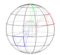
For each bin, a weighted count is accumulated for every neighboring point that lies within. The weight depends on the volume of the bin and the local point density (number of points around the current neighbor). This gives the descriptor some degree of resolution invariance.
We have mentioned that the sphere is given the direction of the normal. This still leaves one degree of freedom (only two axes have been locked, the azimuth remains free). Because of this, the descriptor so far does not cope with rotation. To overcome this (so the same point in two different clouds has the same value), the support sphere is rotated around the normal N times (a number of degrees that corresponds with the divisions in the azimuth) and the process is repeated for each, giving a total of N descriptors for that point.
You can compute the 3DSC descriptor the following way:
#include <pcl/io/pcd_io.h>
#include <pcl/features/normal_3d.h>
#include <pcl/features/3dsc.h>

int
main(int argc, char** argv)
{
	// Object for storing the point cloud.
	pcl::PointCloud<pcl::PointXYZ>::Ptr cloud(new pcl::PointCloud<pcl::PointXYZ>);
	// Object for storing the normals.
	pcl::PointCloud<pcl::Normal>::Ptr normals(new pcl::PointCloud<pcl::Normal>);
	// Object for storing the 3DSC descriptors for each point.
	pcl::PointCloud<pcl::ShapeContext1980>::Ptr descriptors(new pcl::PointCloud<pcl::ShapeContext1980>());

	// Read a PCD file from disk.
	if (pcl::io::loadPCDFile<pcl::PointXYZ>(argv[1], *cloud) != 0)
	{
		return -1;
	}

	// Note: you would usually perform downsampling now. It has been omitted here
	// for simplicity, but be aware that computation can take a long time.

	// Estimate the normals.
	pcl::NormalEstimation<pcl::PointXYZ, pcl::Normal> normalEstimation;
	normalEstimation.setInputCloud(cloud);
	normalEstimation.setRadiusSearch(0.03);
	pcl::search::KdTree<pcl::PointXYZ>::Ptr kdtree(new pcl::search::KdTree<pcl::PointXYZ>);
	normalEstimation.setSearchMethod(kdtree);
	normalEstimation.compute(*normals);

	// 3DSC estimation object.
	pcl::ShapeContext3DEstimation<pcl::PointXYZ, pcl::Normal, pcl::ShapeContext1980> sc3d;
	sc3d.setInputCloud(cloud);
	sc3d.setInputNormals(normals);
	sc3d.setSearchMethod(kdtree);
	// Search radius, to look for neighbors. It will also be the radius of the support sphere.
	sc3d.setRadiusSearch(0.05);
	// The minimal radius value for the search sphere, to avoid being too sensitive
	// in bins close to the center of the sphere.
	sc3d.setMinimalRadius(0.05 / 10.0);
	// Radius used to compute the local point density for the neighbors
	// (the density is the number of points within that radius).
	sc3d.setPointDensityRadius(0.05 / 5.0);

	sc3d.compute(*descriptors);
}
- Input: Points, Normals, Search method, Radius, Minimal radius, Point density radius
- Output: 3DSC descriptors
- Publication:
- Recognizing Objects in Range Data Using Regional Point Descriptors (Andrea Frome et al., 2004)
- API: pcl::ShapeContext3DEstimation
- Download
USC
The Unique Shape Descriptor extends the 3DSC by defining a local reference frame, in order to provide an unique orientation for each point. This not only improves the accuracy of the descriptor, it also reduces its size, as computing multiple descriptors to account for orientation is no longer necessary.
You can check the second publication listed below to learn more about how the LRF is computed.
#include <pcl/io/pcd_io.h>
#include <pcl/features/usc.h>

int
main(int argc, char** argv)
{
	// Object for storing the point cloud.
	pcl::PointCloud<pcl::PointXYZ>::Ptr cloud(new pcl::PointCloud<pcl::PointXYZ>);
	// Object for storing the USC descriptors for each point.
	pcl::PointCloud<pcl::ShapeContext1980>::Ptr descriptors(new pcl::PointCloud<pcl::ShapeContext1980>());

	// Read a PCD file from disk.
	if (pcl::io::loadPCDFile<pcl::PointXYZ>(argv[1], *cloud) != 0)
	{
		return -1;
	}

	// Note: you would usually perform downsampling now. It has been omitted here
	// for simplicity, but be aware that computation can take a long time.

	// USC estimation object.
	pcl::UniqueShapeContext<pcl::PointXYZ, pcl::ShapeContext1980, pcl::ReferenceFrame> usc;
	usc.setInputCloud(cloud);
	// Search radius, to look for neighbors. It will also be the radius of the support sphere.
	usc.setRadiusSearch(0.05);
	// The minimal radius value for the search sphere, to avoid being too sensitive
	// in bins close to the center of the sphere.
	usc.setMinimalRadius(0.05 / 10.0);
	// Radius used to compute the local point density for the neighbors
	// (the density is the number of points within that radius).
	usc.setPointDensityRadius(0.05 / 5.0);
	// Set the radius to compute the Local Reference Frame.
	usc.setLocalRadius(0.05);

	usc.compute(*descriptors);
}
- Input: Points, Radius, Minimal radius, Point density radius, Local radius
- Output: USC descriptors
- Publications:
- Unique Shape Context for 3D Data Description (Federico Tombari et al., 2010)
- Unique Signatures of Histograms for Local Surface Description (Federico Tombari et al., 2010)
- API: pcl::UniqueShapeContext
- Download
SHOT
SHOT stands for Signature of Histograms of Orientations. Like 3DSC, it encodes information about the topology (surface) withing a spherical support structure. This sphere is divided in 32 bins or volumes, with 8 divisions along the azimuth, 2 along the elevation, and 2 along the radius. For every volume, a one-dimensional local histogram is computed. The variable chosen is the angle between the normal of the keypoint and the current point within that volume (to be precise, the cosine, which was found to be better suitable).

When all local histograms have been computed, they are stitched together in a final descriptor. Like the USC descriptor, SHOT makes use of a local reference frame, making it rotation invariant. It is also robust to noise and clutter.
#include <pcl/io/pcd_io.h>
#include <pcl/features/normal_3d.h>
#include <pcl/features/shot.h>

int
main(int argc, char** argv)
{
	// Object for storing the point cloud.
	pcl::PointCloud<pcl::PointXYZ>::Ptr cloud(new pcl::PointCloud<pcl::PointXYZ>);
	// Object for storing the normals.
	pcl::PointCloud<pcl::Normal>::Ptr normals(new pcl::PointCloud<pcl::Normal>);
	// Object for storing the SHOT descriptors for each point.
	pcl::PointCloud<pcl::SHOT352>::Ptr descriptors(new pcl::PointCloud<pcl::SHOT352>());

	// Read a PCD file from disk.
	if (pcl::io::loadPCDFile<pcl::PointXYZ>(argv[1], *cloud) != 0)
	{
		return -1;
	}

	// Note: you would usually perform downsampling now. It has been omitted here
	// for simplicity, but be aware that computation can take a long time.

	// Estimate the normals.
	pcl::NormalEstimation<pcl::PointXYZ, pcl::Normal> normalEstimation;
	normalEstimation.setInputCloud(cloud);
	normalEstimation.setRadiusSearch(0.03);
	pcl::search::KdTree<pcl::PointXYZ>::Ptr kdtree(new pcl::search::KdTree<pcl::PointXYZ>);
	normalEstimation.setSearchMethod(kdtree);
	normalEstimation.compute(*normals);

	// SHOT estimation object.
	pcl::SHOTEstimation<pcl::PointXYZ, pcl::Normal, pcl::SHOT352> shot;
	shot.setInputCloud(cloud);
	shot.setInputNormals(normals);
	// The radius that defines which of the keypoint's neighbors are described.
	// If too large, there may be clutter, and if too small, not enough points may be found.
	shot.setRadiusSearch(0.02);

	shot.compute(*descriptors);
}
Like with FPFH, a multithreading-optimized variant is available with "SHOTEstimationOMP", that makes use of OpenMP. You need to include the header "shot_omp.h". Also, another variant that uses the texture for matching is available, "SHOTColorEstimation", with an optimized version too (see the second publication for more details). It outputs a "SHOT1344" descriptor.
- Input: Points, Normals, Radius
- Output: SHOT descriptors
- Publications:
- Unique Signatures of Histograms for Local Surface Description (Federico Tombari et al., 2010)
- A Combined Texture-Shaped Descriptor for Enhanced 3D Feature Matching (Federico Tombari et al., 2011)
- API: pcl::SHOTEstimation, pcl::SHOTColorEstimation, pcl::SHOTEstimationOMP, pcl::SHOTColorEstimationOMP
- Download
Spin image
The Spin Image (SI) is the oldest descriptor we are going to see here. It has been around since 1997, but it still sees some use for certain applications. It was originally designed to describe surfaces made by vertices, edges and polygons, but it has been since adapted for point clouds. The descriptor is unlike all others in that the output resembles an image that can be compared with another with the usual means.
The support structure used is a cylinder, centered at the point, with a given radius and height, and aligned with the normal. This cylinder is divided radially and vertically into volumes. For each one, the number of neighbors lying inside is added up, eventually producing a descriptor. Weighting and interpolation are used to improve the result. The final descriptor can be seen as a grayscale image where dark areas correspond to volumes with higher point density.

#include <pcl/io/pcd_io.h>
#include <pcl/features/normal_3d.h>
#include <pcl/features/spin_image.h>

// A handy typedef.
typedef pcl::Histogram<153> SpinImage;

int
main(int argc, char** argv)
{
	// Object for storing the point cloud.
	pcl::PointCloud<pcl::PointXYZ>::Ptr cloud(new pcl::PointCloud<pcl::PointXYZ>);
	// Object for storing the normals.
	pcl::PointCloud<pcl::Normal>::Ptr normals(new pcl::PointCloud<pcl::Normal>);
	// Object for storing the spin image for each point.
	pcl::PointCloud<SpinImage>::Ptr descriptors(new pcl::PointCloud<SpinImage>());

	// Read a PCD file from disk.
	if (pcl::io::loadPCDFile<pcl::PointXYZ>(argv[1], *cloud) != 0)
	{
		return -1;
	}

	// Note: you would usually perform downsampling now. It has been omitted here
	// for simplicity, but be aware that computation can take a long time.

	// Estimate the normals.
	pcl::NormalEstimation<pcl::PointXYZ, pcl::Normal> normalEstimation;
	normalEstimation.setInputCloud(cloud);
	normalEstimation.setRadiusSearch(0.03);
	pcl::search::KdTree<pcl::PointXYZ>::Ptr kdtree(new pcl::search::KdTree<pcl::PointXYZ>);
	normalEstimation.setSearchMethod(kdtree);
	normalEstimation.compute(*normals);

	// Spin image estimation object.
	pcl::SpinImageEstimation<pcl::PointXYZ, pcl::Normal, SpinImage> si;
	si.setInputCloud(cloud);
	si.setInputNormals(normals);
	// Radius of the support cylinder.
	si.setRadiusSearch(0.02);
	// Set the resolution of the spin image (the number of bins along one dimension).
	// Note: you must change the output histogram size to reflect this.
	si.setImageWidth(8);

	si.compute(*descriptors);
}
The Spin Image estimation object provides more methods for tuning the estimation, so checking the API is recommended.
- Input: Points, Normals, Radius, Image resolution
- Output: Spin images
- Publications:
- Spin-Images: A Representation for 3-D Surface Matching (Andrew Edie Johnson, 1997)
- Using Spin Images for Efficient Object Recognition in Cluttered 3D Scenes (Andrew Edie Johnson and Martial Hebert, 1999)
- API: pcl::SpinImageEstimation
- Download
RIFT
The Rotation-Invariant Feature Transform, like the spin image, takes some concepts from 2D features, in this case from the Scale-Invariant Feature Transform (SIFT). It is the only descriptor seen here that requires intensity information in order to compute it (it can be obtained from the RGB color values). This means, of course, that you will not be able to use RIFT with standard XYZ clouds, you also need the texture.
In the first step, a circular patch (with the given radius) is fitted on the surface the point lies on. This patch is divided into concentric rings, according to the chosen distance bin size. Then, an histogram is populated with all the point's neighbors lying inside a sphere centered at that point and with the mentioned radius. The distance and the orientation of the intensity gradient at each point are considered. To make it rotation invariant, the angle between the gradient orientation and the vector pointing outward from the center of the patch is measured.
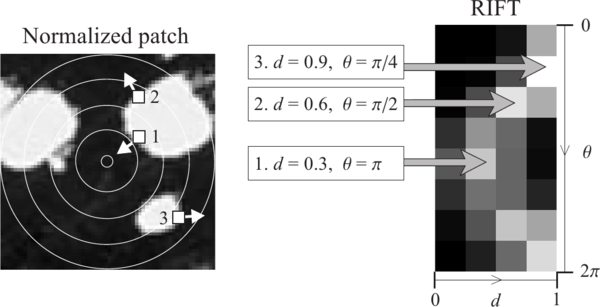
The authors' original implementation uses 4 rings and 8 histogram orientations, which produce a descriptor of size 32. RIFT is not robust to texture flipping, though this was never considered a big issue.
#include <pcl/io/pcd_io.h>
#include <pcl/point_types_conversion.h>
#include <pcl/features/normal_3d.h>
#include <pcl/features/intensity_gradient.h>
#include <pcl/features/rift.h>

// A handy typedef.
typedef pcl::Histogram<32> RIFT32;

int
main(int argc, char** argv)
{
	// Object for storing the point cloud with color information.
	pcl::PointCloud<pcl::PointXYZRGB>::Ptr cloudColor(new pcl::PointCloud<pcl::PointXYZRGB>);
	// Object for storing the point cloud with intensity value.
	pcl::PointCloud<pcl::PointXYZI>::Ptr cloudIntensity(new pcl::PointCloud<pcl::PointXYZI>);
	// Object for storing the intensity gradients.
	pcl::PointCloud<pcl::IntensityGradient>::Ptr gradients(new pcl::PointCloud<pcl::IntensityGradient>);
	// Object for storing the normals.
	pcl::PointCloud<pcl::Normal>::Ptr normals(new pcl::PointCloud<pcl::Normal>);
	// Object for storing the RIFT descriptor for each point.
	pcl::PointCloud<RIFT32>::Ptr descriptors(new pcl::PointCloud<RIFT32>());

	// Read a PCD file from disk.
	if (pcl::io::loadPCDFile<pcl::PointXYZRGB>(argv[1], *cloudColor) != 0)
	{
		return -1;
	}

	// Note: you would usually perform downsampling now. It has been omitted here
	// for simplicity, but be aware that computation can take a long time.

	// Convert the RGB to intensity.
	pcl::PointCloudXYZRGBtoXYZI(*cloudColor, *cloudIntensity);

	// Estimate the normals.
	pcl::NormalEstimation<pcl::PointXYZI, pcl::Normal> normalEstimation;
	normalEstimation.setInputCloud(cloudIntensity);
	normalEstimation.setRadiusSearch(0.03);
	pcl::search::KdTree<pcl::PointXYZI>::Ptr kdtree(new pcl::search::KdTree<pcl::PointXYZI>);
	normalEstimation.setSearchMethod(kdtree);
	normalEstimation.compute(*normals);

	// Compute the intensity gradients.
	pcl::IntensityGradientEstimation < pcl::PointXYZI, pcl::Normal, pcl::IntensityGradient,
		pcl::common::IntensityFieldAccessor<pcl::PointXYZI> > ge;
	ge.setInputCloud(cloudIntensity);
	ge.setInputNormals(normals);
	ge.setRadiusSearch(0.03);
	ge.compute(*gradients);

	// RIFT estimation object.
	pcl::RIFTEstimation<pcl::PointXYZI, pcl::IntensityGradient, RIFT32> rift;
	rift.setInputCloud(cloudIntensity);
	rift.setSearchMethod(kdtree);
	// Set the intensity gradients to use.
	rift.setInputGradient(gradients);
	// Radius, to get all neighbors within.
	rift.setRadiusSearch(0.02);
	// Set the number of bins to use in the distance dimension.
	rift.setNrDistanceBins(4);
	// Set the number of bins to use in the gradient orientation dimension.
	rift.setNrGradientBins(8);
	// Note: you must change the output histogram size to reflect the previous values.

	rift.compute(*descriptors);
}
- Input: Points, Search method, Intensity gradients, Radius, Distance bins, Gradient bins
- Output: RIFT descriptors
- Publication:
- A Sparse Texture Representation Using Local Affine Regions (Svetlana Lazebnik et al., 2005)
- API: pcl::RIFTEstimation, pcl::IntensityGradientEstimation, pcl::IntensityGradient
- Download
NARF
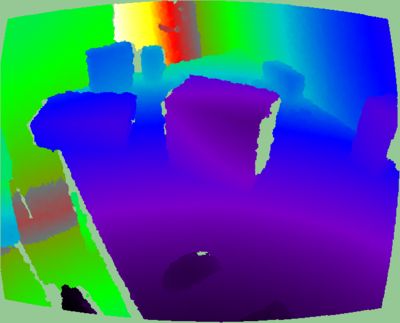
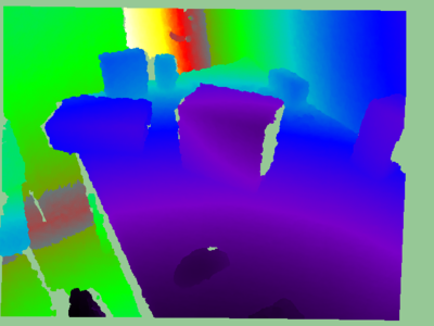
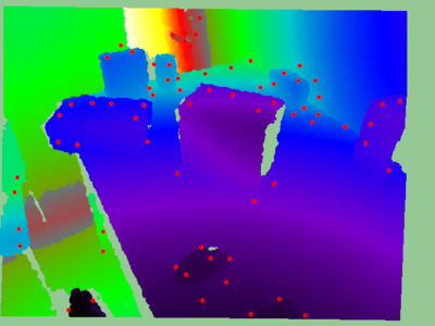
The Normal Aligned Radial Feature is the only descriptor here that does not take a point cloud as input. Instead, it works with range images. A range image is a common RGB image in which the distance to the point that corresponds to a certain pixel is encoded as a color value in the visible light spectrum: the points that are closer to the camera would be violet, while the points near the maximum sensor range would be red.
NARF also requires us to find suitable keypoints to compute the descriptor for. NARF keypoints are located near an object's corners, and this also requires to find the borders (transitions from foreground to background), which are trivial to find with a range image. Because of this lengthy pipeline, I will describe the whole process in different sections.
Obtaining a range image
Because we always work with point clouds, I will now explain how you can convert one into a range image, in order to use it for the NARF descriptor. PCL provides a couple of handy classes to perform the conversion, given that you fill the camera data correctly.
A range image can be created in two ways. First, we can use spherical projection, which would give us an image similar to the ones produced by a LIDAR sensor. Second, we can use planar projection, which is better suitable for camera-like sensors as the Kinect or the Xtion, and will not have the characteristic distortion of the first one.
Spherical projection
The following code will take a point cloud and create a range image from it, using spherical projection:
#include <pcl/io/pcd_io.h>
#include <pcl/range_image/range_image.h>
#include <pcl/visualization/range_image_visualizer.h>

int
main(int argc, char** argv)
{
	// Object for storing the point cloud.
	pcl::PointCloud<pcl::PointXYZ>::Ptr cloud(new pcl::PointCloud<pcl::PointXYZ>);

	// Read a PCD file from disk.
	if (pcl::io::loadPCDFile<pcl::PointXYZ>(argv[1], *cloud) != 0)
	{
		return -1;
	}

	// Parameters needed by the range image object:

	// Angular resolution is the angular distance between pixels.
	// Kinect: 57° horizontal FOV, 43° vertical FOV, 640x480 (chosen here).
	// Xtion: 58° horizontal FOV, 45° vertical FOV, 640x480.
	float angularResolutionX = (float)(57.0f / 640.0f * (M_PI / 180.0f));
	float angularResolutionY = (float)(43.0f / 480.0f * (M_PI / 180.0f));
	// Maximum horizontal and vertical angles. For example, for a full panoramic scan,
	// the first would be 360º. Choosing values that adjust to the real sensor will
	// decrease the time it takes, but don't worry. If the values are bigger than
	// the real ones, the image will be automatically cropped to discard empty zones.
	float maxAngleX = (float)(60.0f * (M_PI / 180.0f));
	float maxAngleY = (float)(50.0f * (M_PI / 180.0f));
	// Sensor pose. Thankfully, the cloud includes the data.
	Eigen::Affine3f sensorPose = Eigen::Affine3f(Eigen::Translation3f(cloud->sensor_origin_[0],
								 cloud->sensor_origin_[1],
								 cloud->sensor_origin_[2])) *
								 Eigen::Affine3f(cloud->sensor_orientation_);
	// Noise level. If greater than 0, values of neighboring points will be averaged.
	// This would set the search radius (i.e., 0.03 == 3cm).
	float noiseLevel = 0.0f;
	// Minimum range. If set, any point closer to the sensor than this will be ignored.
	float minimumRange = 0.0f;
	// Border size. If greater than 0, a border of "unobserved" points will be left
	// in the image when it is cropped.
	int borderSize = 1;

	// Range image object.
	pcl::RangeImage rangeImage;
	rangeImage.createFromPointCloud(*cloud, angularResolutionX, angularResolutionY,
									maxAngleX, maxAngleY, sensorPose, pcl::RangeImage::CAMERA_FRAME,
									noiseLevel, minimumRange, borderSize);

	// Visualize the image.
	pcl::visualization::RangeImageVisualizer viewer("Range image");
	viewer.showRangeImage(rangeImage);
	while (!viewer.wasStopped())
	{
		viewer.spinOnce();
		// Sleep 100ms to go easy on the CPU.
		pcl_sleep(0.1);
	}
}
Here you can see an example of the output range image:
- Input: Points, Angular resolution, Maximum angle, Sensor pose, Coordinate frame, Noise level, Maximum range, Border size
- Output: Range image (spherical projection)
- Tutorials: How to create a range image from a point cloud, How to visualize a range image
- API: pcl::RangeImage
- Download
Planar projection
As mentioned, planar projection will give better results with clouds taken from depth camera:
#include <pcl/io/pcd_io.h>
#include <pcl/range_image/range_image_planar.h>
#include <pcl/visualization/range_image_visualizer.h>

int
main(int argc, char** argv)
{
	// Object for storing the point cloud.
	pcl::PointCloud<pcl::PointXYZ>::Ptr cloud(new pcl::PointCloud<pcl::PointXYZ>);

	// Read a PCD file from disk.
	if (pcl::io::loadPCDFile<pcl::PointXYZ>(argv[1], *cloud) != 0)
	{
		return -1;
	}

	// Parameters needed by the planar range image object:

	// Image size. Both Kinect and Xtion work at 640x480.
	int imageSizeX = 640;
	int imageSizeY = 480;
	// Center of projection. here, we choose the middle of the image.
	float centerX = 640.0f / 2.0f;
	float centerY = 480.0f / 2.0f;
	// Focal length. The value seen here has been taken from the original depth images.
	// It is safe to use the same value vertically and horizontally.
	float focalLengthX = 525.0f, focalLengthY = focalLengthX;
	// Sensor pose. Thankfully, the cloud includes the data.
	Eigen::Affine3f sensorPose = Eigen::Affine3f(Eigen::Translation3f(cloud->sensor_origin_[0],
								 cloud->sensor_origin_[1],
								 cloud->sensor_origin_[2])) *
								 Eigen::Affine3f(cloud->sensor_orientation_);
	// Noise level. If greater than 0, values of neighboring points will be averaged.
	// This would set the search radius (i.e., 0.03 == 3cm).
	float noiseLevel = 0.0f;
	// Minimum range. If set, any point closer to the sensor than this will be ignored.
	float minimumRange = 0.0f;

	// Planar range image object.
	pcl::RangeImagePlanar rangeImagePlanar;
	rangeImagePlanar.createFromPointCloudWithFixedSize(*cloud, imageSizeX, imageSizeY,
			centerX, centerY, focalLengthX, focalLengthX,
			sensorPose, pcl::RangeImage::CAMERA_FRAME,
			noiseLevel, minimumRange);

	// Visualize the image.
	pcl::visualization::RangeImageVisualizer viewer("Planar range image");
	viewer.showRangeImage(rangeImagePlanar);
	while (!viewer.wasStopped())
	{
		viewer.spinOnce();
		// Sleep 100ms to go easy on the CPU.
		pcl_sleep(0.1);
	}
}
- Input: Points, Image size, Projection center, Focal length, Sensor pose, Coordinate frame, Noise level, Maximum range
- Output: Range image (planar projection)
- Tutorials: How to create a range image from a point cloud, How to visualize a range image
- API: pcl::RangeImagePlanar
- Download
If you prefer to do the conversion in real time while you inspect the cloud, PCL ships with an example that fetches an "openni_wrapper::DepthImage" from an OpenNI device and creates the range image from it. You can adapt the code of the example example from tutorial 1 to save it to disk with the function pcl::io::saveRangeImagePlanarFilePNG().
Extracting borders
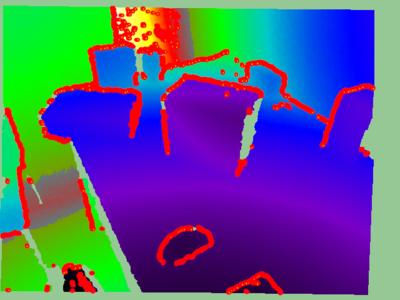
NARF keypoints are located near the edges of objects in the range image, so in order to find them, we first have to extract the borders. A border is defined as an abrupt change from foreground to background. In a range image, this can be easily seen because there is a "jump" in the depth value of two adjacent pixels.
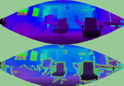
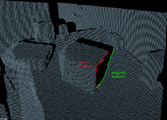
There are three types of borders. Object borders consist of the pixels (or points) located on the very edge of an object (the outermost points still belonging to the object). Shadow borders are points in the background on the edge of occlusions (empty areas in the background due to the objects in front covering them). Notice that, when the cloud is seen from the sensor's viewpoint, object and shadow points will seem adjacent. Finally, veil points are points interpolated between the previous two which appear in scans taken with LIDAR sensors, so we do not have to worry about them here.
Types of borders (image from original paper).
The algorithm basically compares a point's depth with the values of its neighbors, and if a big difference is found, we know it is due to a border. Points closer to the sensor will be marked as object borders, and the other ones as shadow borders.
PCL provides a class for extracting borders of a range image:
#include <pcl/io/pcd_io.h>
#include <pcl/range_image/range_image_planar.h>
#include <pcl/features/range_image_border_extractor.h>
#include <pcl/visualization/range_image_visualizer.h>

int
main(int argc, char** argv)
{
	// Object for storing the point cloud.
	pcl::PointCloud<pcl::PointXYZ>::Ptr cloud(new pcl::PointCloud<pcl::PointXYZ>);
	// Object for storing the borders.
	pcl::PointCloud<pcl::BorderDescription>::Ptr borders(new pcl::PointCloud<pcl::BorderDescription>);

	// Read a PCD file from disk.
	if (pcl::io::loadPCDFile<pcl::PointXYZ>(argv[1], *cloud) != 0)
	{
		return -1;
	}

	// Convert the cloud to range image.
	int imageSizeX = 640, imageSizeY = 480;
	float centerX = (640.0f / 2.0f), centerY = (480.0f / 2.0f);
	float focalLengthX = 525.0f, focalLengthY = focalLengthX;
	Eigen::Affine3f sensorPose = Eigen::Affine3f(Eigen::Translation3f(cloud->sensor_origin_[0],
								 cloud->sensor_origin_[1],
								 cloud->sensor_origin_[2])) *
								 Eigen::Affine3f(cloud->sensor_orientation_);
	float noiseLevel = 0.0f, minimumRange = 0.0f;
	pcl::RangeImagePlanar rangeImage;
	rangeImage.createFromPointCloudWithFixedSize(*cloud, imageSizeX, imageSizeY,
			centerX, centerY, focalLengthX, focalLengthX,
			sensorPose, pcl::RangeImage::CAMERA_FRAME,
			noiseLevel, minimumRange);

	// Border extractor object.
	pcl::RangeImageBorderExtractor borderExtractor(&rangeImage);

	borderExtractor.compute(*borders);

	// Visualize the borders.
	pcl::visualization::RangeImageVisualizer* viewer = NULL;
	viewer = pcl::visualization::RangeImageVisualizer::getRangeImageBordersWidget(rangeImage,
			 -std::numeric_limits<float>::infinity(),
			 std::numeric_limits<float>::infinity(),
			 false, *borders, "Borders");

	while (!viewer->wasStopped())
	{
		viewer->spinOnce();
		// Sleep 100ms to go easy on the CPU.
		pcl_sleep(0.1);
	}
}
You can use the extractor's "getParameters()" function to get a pcl::RangeImageBorderExtractor::Parameters struct with the settings that will be used.
- Input: Range image
- Output: Borders
- Tutorial: How to extract borders from range images
- Publication:
- Point Feature Extraction on 3D Range Scans Taking into Account Object Boundaries (Bastian Steder et al., 2011)
- API: pcl::RangeImageBorderExtractor
- Download
Finding keypoints
Citing the original publication:
"We have the following requirements for our interest point extraction procedure:
- It must take information about borders and the surface structure into account.
- It must select positions that can be reliably detected even if the object is observed from another perspective.
- The points must be on positions that provide stable areas for normal estimation or the descriptor calculation in general.
The procedure is the following: for every point in the range image, a score is computed that conveys how much the surface changes in its neighborhood (this is tuned with the support size σ, which is the diameter of the sphere used to find neighboring points). Also, the dominant direction of this change is computed. Then, this direction is compared with those of the neighbors, trying to find how stable the point is (if the directions are very different, that means the point is not stable, and that the surface around changes a lot). Points that are near the object's corners (but not exactly on the very edge) will be good keypoints, yet stable enough.
NARF keypoints (image from original paper).
Interest regions with a support size of 20cm (up) and 1m (down) (image from original paper).
In PCL, NARF keypoints can be found this way:
#include <pcl/io/pcd_io.h>
#include <pcl/range_image/range_image_planar.h>
#include <pcl/features/range_image_border_extractor.h>
#include <pcl/keypoints/narf_keypoint.h>
#include <pcl/visualization/range_image_visualizer.h>

int
main(int argc, char** argv)
{
	// Object for storing the point cloud.
	pcl::PointCloud<pcl::PointXYZ>::Ptr cloud(new pcl::PointCloud<pcl::PointXYZ>);
	// Object for storing the keypoints' indices.
	pcl::PointCloud<int>::Ptr keypoints(new pcl::PointCloud<int>);

	// Read a PCD file from disk.
	if (pcl::io::loadPCDFile<pcl::PointXYZ>(argv[1], *cloud) != 0)
	{
		return -1;
	}

	// Convert the cloud to range image.
	int imageSizeX = 640, imageSizeY = 480;
	float centerX = (640.0f / 2.0f), centerY = (480.0f / 2.0f);
	float focalLengthX = 525.0f, focalLengthY = focalLengthX;
	Eigen::Affine3f sensorPose = Eigen::Affine3f(Eigen::Translation3f(cloud->sensor_origin_[0],
								 cloud->sensor_origin_[1],
								 cloud->sensor_origin_[2])) *
								 Eigen::Affine3f(cloud->sensor_orientation_);
	float noiseLevel = 0.0f, minimumRange = 0.0f;
	pcl::RangeImagePlanar rangeImage;
	rangeImage.createFromPointCloudWithFixedSize(*cloud, imageSizeX, imageSizeY,
			centerX, centerY, focalLengthX, focalLengthX,
			sensorPose, pcl::RangeImage::CAMERA_FRAME,
			noiseLevel, minimumRange);

	pcl::RangeImageBorderExtractor borderExtractor;
	// Keypoint detection object.
	pcl::NarfKeypoint detector(&borderExtractor);
	detector.setRangeImage(&rangeImage);
	// The support size influences how big the surface of interest will be,
	// when finding keypoints from the border information.
	detector.getParameters().support_size = 0.2f;

	detector.compute(*keypoints);

	// Visualize the keypoints.
	pcl::visualization::RangeImageVisualizer viewer("NARF keypoints");
	viewer.showRangeImage(rangeImage);
	for (size_t i = 0; i < keypoints->points.size(); ++i)
	{
		viewer.markPoint(keypoints->points[i] % rangeImage.width,
						 keypoints->points[i] / rangeImage.width,
						 // Set the color of the pixel to red (the background
						 // circle is already that color). All other parameters
						 // are left untouched, check the API for more options.
						 pcl::visualization::Vector3ub(1.0f, 0.0f, 0.0f));
	}

	while (!viewer.wasStopped())
	{
		viewer.spinOnce();
		// Sleep 100ms to go easy on the CPU.
		pcl_sleep(0.1);
	}
}
- Input: Range image, Border extractor, Support Size
- Output: NARF keypoints
- Tutorial: How to extract NARF keypoint from a range image
- Publication:
- Point Feature Extraction on 3D Range Scans Taking into Account Object Boundaries (Bastian Steder et al., 2011)
- API: pcl::NarfKeypoint
- Download
Computing the descriptor
We have created the range image from a point cloud, and we have extracted the borders in order to find good keypoints. Now it is time to compute the NARF descriptor for each keypoint.
The NARF descriptor encodes information about surface changes around a point. First, a local range patch is created around the point. It is like a small range image centered at that point, aligned with the normal (it would seem as if we were looking at the point along the normal). Then, a star pattern with n beams is overlaid onto the patch, also centered at the point. For every beam, a value is computed, that reflects how much the surface under it changes. The stronger the change is, and the closer to the center it is, the higher the final value will be. The n resulting values compose the final descriptor.
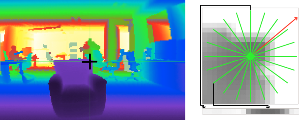
The descriptor right now is not invariant to rotations around the normal. To achieve this, the whole possible 360 degrees are binned into an histogram. The value of each bin is computed from the descriptor values according the the angle. Then, the bin with the highest value is considered the dominant orientation, and the descriptor is shifted according to it.
#include <pcl/io/pcd_io.h>
#include <pcl/range_image/range_image_planar.h>
#include <pcl/features/range_image_border_extractor.h>
#include <pcl/keypoints/narf_keypoint.h>
#include <pcl/features/narf_descriptor.h>

int
main(int argc, char** argv)
{
	// Object for storing the point cloud.
	pcl::PointCloud<pcl::PointXYZ>::Ptr cloud(new pcl::PointCloud<pcl::PointXYZ>);
	// Object for storing the keypoints' indices.
	pcl::PointCloud<int>::Ptr keypoints(new pcl::PointCloud<int>);
	// Object for storing the NARF descriptors.
	pcl::PointCloud<pcl::Narf36>::Ptr descriptors(new pcl::PointCloud<pcl::Narf36>);

	// Read a PCD file from disk.
	if (pcl::io::loadPCDFile<pcl::PointXYZ>(argv[1], *cloud) != 0)
	{
		return -1;
	}

	// Convert the cloud to range image.
	int imageSizeX = 640, imageSizeY = 480;
	float centerX = (640.0f / 2.0f), centerY = (480.0f / 2.0f);
	float focalLengthX = 525.0f, focalLengthY = focalLengthX;
	Eigen::Affine3f sensorPose = Eigen::Affine3f(Eigen::Translation3f(cloud->sensor_origin_[0],
								 cloud->sensor_origin_[1],
								 cloud->sensor_origin_[2])) *
								 Eigen::Affine3f(cloud->sensor_orientation_);
	float noiseLevel = 0.0f, minimumRange = 0.0f;
	pcl::RangeImagePlanar rangeImage;
	rangeImage.createFromPointCloudWithFixedSize(*cloud, imageSizeX, imageSizeY,
			centerX, centerY, focalLengthX, focalLengthX,
			sensorPose, pcl::RangeImage::CAMERA_FRAME,
			noiseLevel, minimumRange);

	// Extract the keypoints.
	pcl::RangeImageBorderExtractor borderExtractor;
	pcl::NarfKeypoint detector(&borderExtractor);
	detector.setRangeImage(&rangeImage);
	detector.getParameters().support_size = 0.2f;
	detector.compute(*keypoints);

	// The NARF estimator needs the indices in a vector, not a cloud.
	std::vector<int> keypoints2;
	keypoints2.resize(keypoints->points.size());
	for (unsigned int i = 0; i < keypoints->size(); ++i)
		keypoints2[i] = keypoints->points[i];
	// NARF estimation object.
	pcl::NarfDescriptor narf(&rangeImage, &keypoints2);
	// Support size: choose the same value you used for keypoint extraction.
	narf.getParameters().support_size = 0.2f;
	// If true, the rotation invariant version of NARF will be used. The histogram
	// will be shifted according to the dominant orientation to provide robustness to
	// rotations around the normal.
	narf.getParameters().rotation_invariant = true;

	narf.compute(*descriptors);
}
- Input: Range image, Key points, Support Size
- Output: NARF descriptors
- Tutorial: How to extract NARF Features from a range image
- Publication:
- Point Feature Extraction on 3D Range Scans Taking into Account Object Boundaries (Bastian Steder et al., 2011)
- API: pcl::NarfDescriptor
- Download
Global descriptors
Global descriptors encode object geometry. They are not computed for individual points, but for a whole cluster that represents an object. Because of this, a preprocessing step (segmentation) is required, in order to retrieve possible candidates.
Global descriptors are used for object recognition and classification, geometric analysis (object type, shape...), and pose estimation.
You should also know that many local descriptors can also be used as global ones. This can be done with descriptors that use a radius to search for neighbors (as PFH does). The trick is to compute it for one single point in the object cluster, and set the radius to the maximum possible distance between any two points (so all points in the cluster are considered as neighbors).
VFH
The Viewpoint Feature Histogram is based on the FPFH. Because the latter is invariant to the object's pose, the authors decided to expand it by including information about the viewpoint. Also, the FPFH is estimated once for the whole cluster, not for every point.
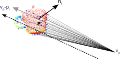
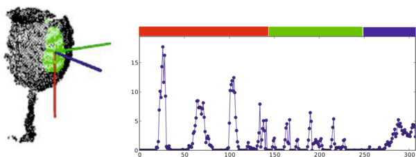
The VFH is made up by two parts: a viewpoint direction component, and an extended FPFH component. To compute the first one, the object's centroid is found, which is the point that results from averaging the X, Y and Z coordinates of all points. Then, the vector between the viewpoint (the position of the sensor) and this centroid is computed, and normalized. Finally, for all points in the cluster, the angle between this vector and their normal is calculated, and the result is binned into an histogram. The vector is translated to each point when computing the angle because it makes the descriptor scale invariant.
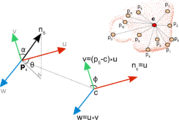
The second component is computed like the FPFH (that results in 3 histograms for the 3 angular features, α, φ and θ), with some differences: it is only computed for the centroid, using the computed viewpoint direction vector as its normal (as the point, obviously, does not have a normal), and setting all the cluster's points as neighbors.
Viewpoint component of the VFH (image from original paper).
Extended FPFH component of the VFH (image from original paper).
The resulting 4 histograms (1 for the viewpoint component, 3 for the extended FPFH component) are concatenated to build the final VFH descriptor. By default, the bins are normalized using the total number of points in the cluster. This makes the VFH descriptor invariant to scale.
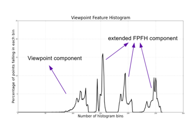
The PCL implementation computes an additional fifth histogram with the distances of the cluster points to the centroid (the Shape Distribution Component, SDC), increading the size of the output descriptor from 263 to 308. The SDC is taken from the CVFH descriptor that we will see in the next section, and makes the result more robust.
The VFH of an already clustered object can be computed this way:
#include <pcl/io/pcd_io.h>
#include <pcl/features/normal_3d.h>
#include <pcl/features/vfh.h>

int
main(int argc, char** argv)
{
	// Cloud for storing the object.
	pcl::PointCloud<pcl::PointXYZ>::Ptr object(new pcl::PointCloud<pcl::PointXYZ>);
	// Object for storing the normals.
	pcl::PointCloud<pcl::Normal>::Ptr normals(new pcl::PointCloud<pcl::Normal>);
	// Object for storing the VFH descriptor.
	pcl::PointCloud<pcl::VFHSignature308>::Ptr descriptor(new pcl::PointCloud<pcl::VFHSignature308>);

	// Note: you should have performed preprocessing to cluster out the object
	// from the cloud, and save it to this individual file.

	// Read a PCD file from disk.
	if (pcl::io::loadPCDFile<pcl::PointXYZ>(argv[1], *object) != 0)
	{
		return -1;
	}

	// Estimate the normals.
	pcl::NormalEstimation<pcl::PointXYZ, pcl::Normal> normalEstimation;
	normalEstimation.setInputCloud(object);
	normalEstimation.setRadiusSearch(0.03);
	pcl::search::KdTree<pcl::PointXYZ>::Ptr kdtree(new pcl::search::KdTree<pcl::PointXYZ>);
	normalEstimation.setSearchMethod(kdtree);
	normalEstimation.compute(*normals);

	// VFH estimation object.
	pcl::VFHEstimation<pcl::PointXYZ, pcl::Normal, pcl::VFHSignature308> vfh;
	vfh.setInputCloud(object);
	vfh.setInputNormals(normals);
	vfh.setSearchMethod(kdtree);
	// Optionally, we can normalize the bins of the resulting histogram,
	// using the total number of points.
	vfh.setNormalizeBins(true);
	// Also, we can normalize the SDC with the maximum size found between
	// the centroid and any of the cluster's points.
	vfh.setNormalizeDistance(false);

	// Compute the features
	vfh.compute(*descriptor);
}
Because only one VFH descriptor is computed for the whole cluster, the size of the cloud object that stores the result will be 1.
- Input: Points (cluster), Normals, Search method, [Normalize bins], [Normalize SDC]
- Output: VFH descriptor
- Tutorial: Estimating VFH signatures for a set of points
- Publication:
- Fast 3D Recognition and Pose Using the Viewpoint Feature Histogram (Radu Bogdan Rusu et al., 2010)
- API: pcl::VFHEstimation
- Download
CVFH
The original VFH descriptor is not robust to occlusion or other sensor artifacts, or measurement errors. If the object cluster is missing many points, the resulting computed centroid will differ from the original, altering the final descriptor, and preventing a positive match from being found. Because of that, the Clustered Viewpoint Feature Histogram (CVFH) was introduced.
The idea is very simple: instead of computing a single VFH histogram for the whole cluster, the object is first divided in stable, smooth regions using region-growing segmentation, that enforces several constraints in the distances and differences of normals of the points belonging to every region. Then, a VFH is computed for every region. Thanks to this, an object can be found in a scene, as long as at least one of its regions is fully visible.
Typical occlusion issues in a point cloud (image from original paper).
Object regions computed for the CVFH (image from original paper).
Additionally, a Shape Distribution Component (SDC) is also computed and included. It encodes information about the distribution of the points arond the region's centroid, measuring the distances. The SDC allows to differentiate objects with similar characteristics (size and normal distribution), like two planar surfaces from each other.
The authors proposed to discard the histogram normalization step that is performed in VFH. This has the effect of making the descriptor dependant of scale, so an object of a certain size would not match a bigger or smaller copy of itself. It also makes CVFH more robust to occlusion.
CVFH is invariant to the camera roll angle. The use of a Camera Roll Histogram (CRH) has been proposed to overcome this.
#include <pcl/io/pcd_io.h>
#include <pcl/features/normal_3d.h>
#include <pcl/features/cvfh.h>

int
main(int argc, char** argv)
{
	// Cloud for storing the object.
	pcl::PointCloud<pcl::PointXYZ>::Ptr object(new pcl::PointCloud<pcl::PointXYZ>);
	// Object for storing the normals.
	pcl::PointCloud<pcl::Normal>::Ptr normals(new pcl::PointCloud<pcl::Normal>);
	// Object for storing the CVFH descriptors.
	pcl::PointCloud<pcl::VFHSignature308>::Ptr descriptors(new pcl::PointCloud<pcl::VFHSignature308>);

	// Note: you should have performed preprocessing to cluster out the object
	// from the cloud, and save it to this individual file.

	// Read a PCD file from disk.
	if (pcl::io::loadPCDFile<pcl::PointXYZ>(argv[1], *object) != 0)
	{
		return -1;
	}

	// Estimate the normals.
	pcl::NormalEstimation<pcl::PointXYZ, pcl::Normal> normalEstimation;
	normalEstimation.setInputCloud(object);
	normalEstimation.setRadiusSearch(0.03);
	pcl::search::KdTree<pcl::PointXYZ>::Ptr kdtree(new pcl::search::KdTree<pcl::PointXYZ>);
	normalEstimation.setSearchMethod(kdtree);
	normalEstimation.compute(*normals);

	// CVFH estimation object.
	pcl::CVFHEstimation<pcl::PointXYZ, pcl::Normal, pcl::VFHSignature308> cvfh;
	cvfh.setInputCloud(object);
	cvfh.setInputNormals(normals);
	cvfh.setSearchMethod(kdtree);
	// Set the maximum allowable deviation of the normals,
	// for the region segmentation step.
	cvfh.setEPSAngleThreshold(5.0 / 180.0 * M_PI); // 5 degrees.
	// Set the curvature threshold (maximum disparity between curvatures),
	// for the region segmentation step.
	cvfh.setCurvatureThreshold(1.0);
	// Set to true to normalize the bins of the resulting histogram,
	// using the total number of points. Note: enabling it will make CVFH
	// invariant to scale just like VFH, but the authors encourage the opposite.
	cvfh.setNormalizeBins(false);

	// Compute the features
	cvfh.compute(*descriptors);
}
You can further customize the segmentation step with "setClusterTolerance()" (to set the maximum Euclidean distance between points in the same cluster) and "setMinPoints()". The size of the output will be equal to the number of regions the object was divided in.
- Input: Points (cluster), Normals, Search method, Angle threshold, Curvature threshold, [Normalize bins], [Cluster tolerance], [Minimum points]
- Output: CVFH descriptors
- Publication:
- CAD-Model Recognition and 6DOF Pose Estimation Using 3D Cues (requires IEEE Xplore subscription) (Aitor Aldoma et al., 2011)
- API: pcl::CVFHEstimation
- Download
OUR-CVFH
The Oriented, Unique and Repeatable CVFH expands the previous descriptor, adding the computation of an unique reference frame to make it more robust.
OUR-CVFH relies on the use of Semi-Global Unique Reference Frames (SGURFs), which are repeatable coordinate systems computed for each region. Not only the remove the invariance to camera roll and allow to extract the 6DoF pose directly without additional steps, but they also improve the spatial descriptiveness.
The first part of the computation is akin to CVFH, but after segmentation, the points in each region are filtered once more according to the difference between their normals and the region's average normal. This results in better shaped regions, improving the estimation of the Reference Frames (RFs).
After this, the SGURF is computed for each region. Disambiguation is performed to decide the sign of the axes, according to the points' distribution. If this is not enough and the sign remains ambiguous, multiple RFs will need to be created to account for it. Finally, the OUR-CVFH descriptor is computed. The original Shape Distribution Component (SDC) is discarded, and the surface is now described according to the RFs.
#include <pcl/io/pcd_io.h>
#include <pcl/features/normal_3d.h>
#include <pcl/features/our_cvfh.h>

int
main(int argc, char** argv)
{
	// Cloud for storing the object.
	pcl::PointCloud<pcl::PointXYZ>::Ptr object(new pcl::PointCloud<pcl::PointXYZ>);
	// Object for storing the normals.
	pcl::PointCloud<pcl::Normal>::Ptr normals(new pcl::PointCloud<pcl::Normal>);
	// Object for storing the OUR-CVFH descriptors.
	pcl::PointCloud<pcl::VFHSignature308>::Ptr descriptors(new pcl::PointCloud<pcl::VFHSignature308>);

	// Note: you should have performed preprocessing to cluster out the object
	// from the cloud, and save it to this individual file.

	// Read a PCD file from disk.
	if (pcl::io::loadPCDFile<pcl::PointXYZ>(argv[1], *object) != 0)
	{
		return -1;
	}

	// Estimate the normals.
	pcl::NormalEstimation<pcl::PointXYZ, pcl::Normal> normalEstimation;
	normalEstimation.setInputCloud(object);
	normalEstimation.setRadiusSearch(0.03);
	pcl::search::KdTree<pcl::PointXYZ>::Ptr kdtree(new pcl::search::KdTree<pcl::PointXYZ>);
	normalEstimation.setSearchMethod(kdtree);
	normalEstimation.compute(*normals);

	// OUR-CVFH estimation object.
	pcl::OURCVFHEstimation<pcl::PointXYZ, pcl::Normal, pcl::VFHSignature308> ourcvfh;
	ourcvfh.setInputCloud(object);
	ourcvfh.setInputNormals(normals);
	ourcvfh.setSearchMethod(kdtree);
	ourcvfh.setEPSAngleThreshold(5.0 / 180.0 * M_PI); // 5 degrees.
	ourcvfh.setCurvatureThreshold(1.0);
	ourcvfh.setNormalizeBins(false);
	// Set the minimum axis ratio between the SGURF axes. At the disambiguation phase,
	// this will decide if additional Reference Frames need to be created, if ambiguous.
	ourcvfh.setAxisRatio(0.8);

	// Compute the features
	ourcvfh.compute(*descriptors);
}
- Input: Points (cluster), Normals, Search method, Angle threshold, Curvature threshold, [Normalize bins], [Cluster tolerance], [Minimum points], [Axis ratio]
- Output: OUR-CVFH descriptors
- Publication:
- API: pcl::OURCVFHEstimation
- Download
ESF
The Ensemble of Shape Functions (ESF) is a combination of 3 different shape functions that describe certain properties of the cloud's points: distances, angles and area. This descriptor is very unique because it does not require normal information. Actually, it does not need any preprocessing, as it is robust to noise and incomplete surfaces.
The algorithm uses a voxel grid as an approximation of the real surface. It iterates through all the points in the cloud: for every iteration, 3 random points are chosen. For these points, the shape functions are computed:
- D2: this function computes the distances between point pairs (3 overall). Then, for every pair, it checks if the line that connects both points lies entirely inside the surface, entirely outside (crossing free space), or both. Depending on this, the distance value will be binned to one of three possible histograms: IN, OUT or MIXED.
- D2 ratio: an additional histogram for the ratio between parts of the line inside the surface, and parts outside. This value will be 0 if the line is completely outside, 1 if completely inside, and some value in between if mixed.
- D3: this computes the square root of the area of the triangle formed by the 3 points. Like D2, the result is also classified as IN, OUT or MIXED, each with its own histogram.
- A3: this function computes the angle formed by the points. Then, the value is binned depending on how the line opposite to the angle is (once again, as IN, OUT or MIXED).

After the loop is over, we are left with 10 subhistograms (IN, OUT and MIXED for D2, D3 and A3, and an additional one for the ratio). Each one has 64 bins, so the size of the final ESF descriptor is 640.
#include <pcl/io/pcd_io.h>
#include <pcl/features/esf.h>

int
main(int argc, char** argv)
{
	// Cloud for storing the object.
	pcl::PointCloud<pcl::PointXYZ>::Ptr object(new pcl::PointCloud<pcl::PointXYZ>);
	// Object for storing the ESF descriptor.
	pcl::PointCloud<pcl::ESFSignature640>::Ptr descriptor(new pcl::PointCloud<pcl::ESFSignature640>);

	// Note: you should have performed preprocessing to cluster out the object
	// from the cloud, and save it to this individual file.

	// Read a PCD file from disk.
	if (pcl::io::loadPCDFile<pcl::PointXYZ>(argv[1], *object) != 0)
	{
		return -1;
	}

	// ESF estimation object.
	pcl::ESFEstimation<pcl::PointXYZ, pcl::ESFSignature640> esf;
	esf.setInputCloud(object);

	// Compute the features
	esf.compute(*descriptor);
}
- Input: Points (cluster)
- Output: ESF descriptor
- Publication:
- Ensemble of shape functions for 3D object classification (requires IEEE Xplore subscription) (Walter Wohlkinger and Markus Vincze, 2011)
- API: pcl::ESFEstimation
- Download
GFPFH
As you may have guessed, GFPFH stands for Global Fast Point Feature Histogram, the global version of the FPFH descriptor. GFPFH was designed for the task of helping a robot navigate its environment, having some context of the objects around it.
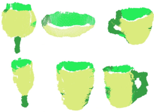
The first step before being able to compute the descriptor is surface categorization. A set of logical primitives (the classes, or categories) is created, which depends on the type of objects we expect the robot to find on the scene. For example, if we know there will be a coffee mug, we create three: one for the handle, and the other two for the outer and inner faces. Then, FPFH descriptors are computed, and everything is fed to a Conditional Random Field (CRF) algorithm. The CRF will label each surface with one of the previous categories, so we end up with a cloud where each point has been classified depending of the type of object (or object's region) it belongs to.
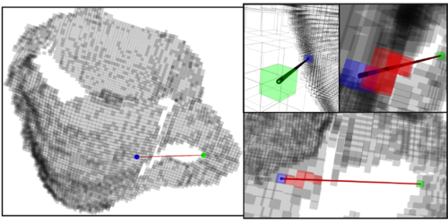
Now, the GFPFH descriptor can be computed with the result of the classification step. It will encode what the object is made of, so the robot can easily recognize it. First, an octree is created, dividing the object in voxel leaves. For every leaf, a set of probabilities is created, one for each class. Each one stores the probability of that leaf belonging to the class, and it is computed according to the number of points in that leaf that have been labelled as that class, and the total number of points. Then, for every pair of leaves in the octree, a line is casted, connecting them. Every leaf in its path is checked for occupancy, storing the result in an histogram. If the leaf is empty (free space), a value of 0 is saved. Otherwise, the leaf probabilities are used.
The following code will compute the GFPFH for a cloud with label information. The categorization step is up to you, as it depends largely on the type of the scene, and the use you are going to give it.
#include <pcl/io/pcd_io.h>
#include <pcl/features/gfpfh.h>

int
main(int argc, char** argv)
{
	// Cloud for storing the object.
	pcl::PointCloud<pcl::PointXYZL>::Ptr object(new pcl::PointCloud<pcl::PointXYZL>);
	// Object for storing the GFPFH descriptor.
	pcl::PointCloud<pcl::GFPFHSignature16>::Ptr descriptor(new pcl::PointCloud<pcl::GFPFHSignature16>);

	// Note: you should have performed preprocessing to cluster out the object
	// from the cloud, and save it to this individual file.

	// Read a PCD file from disk.
	if (pcl::io::loadPCDFile<pcl::PointXYZL>(argv[1], *object) != 0)
	{
		return -1;
	}

	// Note: you should now perform classification on the cloud's points. See the
	// original paper for more details. For this example, we will now consider 4
	// different classes, and randomly label each point as one of them.
	for (size_t i = 0; i < object->points.size(); ++i)
	{
		object->points[i].label = 1 + i % 4;
	}

	// ESF estimation object.
	pcl::GFPFHEstimation<pcl::PointXYZL, pcl::PointXYZL, pcl::GFPFHSignature16> gfpfh;
	gfpfh.setInputCloud(object);
	// Set the object that contains the labels for each point. Thanks to the
	// PointXYZL type, we can use the same object we store the cloud in.
	gfpfh.setInputLabels(object);
	// Set the size of the octree leaves to 1cm (cubic).
	gfpfh.setOctreeLeafSize(0.01);
	// Set the number of classes the cloud has been labelled with (default is 16).
	gfpfh.setNumberOfClasses(4);

	// Compute the features
	gfpfh.compute(*descriptor);
}
- Input: Points (cluster), Labels, Number of classes, Leaf size
- Output: GFPFH descriptor
- Publication:
- Detecting and Segmenting Objects for Mobile Manipulation (Radu Bogdan Rusu et al., 2009)
- API: pcl::GFPFHEstimation
- Download
GRSD
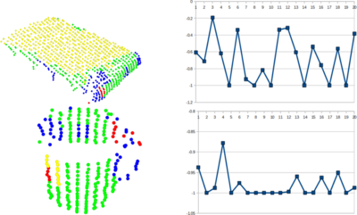
The global version of the Radius-based Surface Descriptor works in a similar fashion to GFPFH. A voxelization and a surface categorization step are performed beforehand, labelling all surface patches according to the geometric category (plane, cylinder, edge, rim, sphere), using RSD. Then, the whole cluster is classified into one of these categories, and the GRSD descriptor is computed from this.
As with RSD, I will provide a code snippet when the descriptor becomes available in PCL.
- Publication:
- Hierarchical Object Geometric Categorization and Appearance Classification for Mobile Manipulation (Zoltan-Csaba Marton et al., 2010)
Visualization
Sometimes it is desired to check a visual representation of a descriptor, perhaps to analyze the distribution of data over different bins. Because they are saved as histograms, this is something trivial to do. PCL offers a couple of classes to do this.
Histogram Visualizer
"PCLHistogramVisualizer" is the simplest way to plot an histogram. The class has little functionality, but it does its job. Only one call is necessary to give the histogram and its size:
#include <pcl/io/pcd_io.h>
#include <pcl/features/normal_3d.h>
#include <pcl/features/vfh.h>
#include<pcl/visualization/histogram_visualizer.h>

int
main(int argc, char** argv)
{
	// Clouds for storing everything.
	pcl::PointCloud<pcl::PointXYZ>::Ptr object(new pcl::PointCloud<pcl::PointXYZ>);
	pcl::PointCloud<pcl::Normal>::Ptr normals(new pcl::PointCloud<pcl::Normal>);
	pcl::PointCloud<pcl::VFHSignature308>::Ptr descriptor(new pcl::PointCloud<pcl::VFHSignature308>);

	// Read a PCD file from disk.
	if (pcl::io::loadPCDFile<pcl::PointXYZ>(argv[1], *object) != 0)
	{
		return -1;
	}

	// Estimate the normals.
	pcl::NormalEstimation<pcl::PointXYZ, pcl::Normal> normalEstimation;
	normalEstimation.setInputCloud(object);
	normalEstimation.setRadiusSearch(0.03);
	pcl::search::KdTree<pcl::PointXYZ>::Ptr kdtree(new pcl::search::KdTree<pcl::PointXYZ>);
	normalEstimation.setSearchMethod(kdtree);
	normalEstimation.compute(*normals);

	// Estimate VFH descriptor.
	pcl::VFHEstimation<pcl::PointXYZ, pcl::Normal, pcl::VFHSignature308> vfh;
	vfh.setInputCloud(object);
	vfh.setInputNormals(normals);
	vfh.setSearchMethod(kdtree);
	vfh.setNormalizeBins(true);
	vfh.setNormalizeDistance(false);
	vfh.compute(*descriptor);

	// Plotter object.
	pcl::visualization::PCLHistogramVisualizer viewer;
	// We need to set the size of the descriptor beforehand.
	viewer.addFeatureHistogram(*descriptor, 308);

	viewer.spin();
}
- Input: Descriptor, descriptor size, [Window size], [Background color], [Y axis range]
- API: pcl::visualization::PCLHistogramVisualizer
- Download
PCL Viewer
This program, included with PCL, will also let you open and visualize a saved descriptor. Remember that you can save a descriptor to a file just like with any other cloud type. Once done, invoke the viewer from the command line:
pcl_viewer <descriptor_file>
Go to root: PhD-3D-Object-Tracking
Links to articles:
PCL/OpenNI tutorial 0: The very basics
PCL/OpenNI tutorial 1: Installing and testing
PCL/OpenNI tutorial 2: Cloud processing (basic)
PCL/OpenNI tutorial 3: Cloud processing (advanced)
PCL/OpenNI tutorial 4: 3D object recognition (descriptors)
