PCL/OpenNI tutorial 2: Cloud processing (basic)
Go to root: PhD-3D-Object-Tracking
All right: in the previous tutorial you installed OpenNI and PCL. You managed to get your device working. You compiled and ran the example program, watched as it fetched one frame after another, and even saved a couple of point clouds to disk. Now you may be wondering "What about now? What use depth sensors are? What can I do with point clouds?"
Well, depth cameras have a lot of useful applications. For example, you could use them as motion tracking hardware and save you thousands of dollars in professional gear. The original Kinect was actually designed as an alternative to physical controllers (i.e., gamepads) in games. Hand gestures can also be recognized, so people have managed to successfully implement control interfaces similar to what could be seen in Minority Report.
Working low-level with point clouds offers interesting possibilities too. As they are essentially a 3D "scan" or the scene, you could capture your whole room as a continuous 3D mesh, then import it in your modelling software of choice and use it as a reference for a better reconstruction. You could use it to measure distances, or detect obstacles, for a robot navigation system. But the most exciting alternative by far, and the one where most of the research is being focused on, is to perform 3D object recognition and pose estimation, even in real time. This allows a robot to fulfill tasks like going to the kitchen to get you a cup of coffee.
Most of the advanced stuff that can be done with a point cloud requires some previous steps, like filtering, reconstruction or normal estimation. In this tutorial, I will introduce you to the basics of point cloud processing, and leave the complicated methods for the next tutorial. I will explain what every technique does and what it should be used for, and include PCL code snippets so you can check how to implement it in your programs.
Point clouds
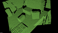
First, a little explanation. A point cloud as taken from a depth sensor consists of a series of points in 3D space, as simple as that. A "pcl::PointCloud<PointT>" object stores the points inside a "std::vector<PointT>" structure. The cloud object exposes some functions that let you get information about them, like the point count. As you can see, the class is templated so you can instantiate it for many types of points. For example, "PointXYZ", which stores three floats for the X, Y and Z coordinates, and "PointXYZRGB", which also stores color (texture) information for each point, the kind we would get with Kinect or Xtion RGB-D cameras. A list of point types and a basic description of the cloud object are available on PCL's website.
Clouds will usually be handled with pointers, as they tend to be large. PCL implements the "boost::shared_ptr" class from Boost C++ libraries, that keeps track of the references to a certain object. Every time you pass a shared pointer and a copy of it is created, a reference counter is automatically increased. When the pointer is destroyed, it is decreased. If the counter ever reaches 0, it means that no one is holding an active reference to the object, and its destructor is called to free memory. This can take a while to get used to, and you will be mixing cloud objects and cloud object pointers until then, but do not worry.
PCD files
When clouds are saved to disk, a PCD (Point Cloud Data) file is produced. You can choose to do it so in binary or plain text format. The first one is faster to work with, whereas the second one will let you to inspect the cloud by opening it with a common text editor. If you do so, you may see something like this:
# .PCD v.7 − Point Cloud Data file format
VERSION .7
FIELDS x y z
SIZE 4 4 4
TYPE F F F
WIDTH 2
HEIGHT 1
VIEWPOINT 0 0 0 1 0 0 0
POINTS 2
DATA ascii
0.73412 -1.12643 0.82218
0.44739 -0.34735 -0.04624
This tells us that the cloud consist of 2 points of type "PointXYZ" (because each point has only 3 fields; the X, Y and Z coordinates, each stored in a 4-byte float), and lists their coordinates. It also stores the viewport information (the relative position of the points to the sensor) as a translation quaternion. Knowing the position of the camera can be useful for certain procedures like normal estimation.
Reading from file
Reading a point cloud from a PCD file to and storing it in memory can be done with a single function call. You must specify the correct point type. For example, for .pcd files saved with the OpenNI viewer application that we saw in the previous tutorial, you could use either "PointXYZRGBA" or "PointXYZ" if you are not going to use the color information.
#include <pcl/io/pcd_io.h>

int
main(int argc, char** argv)
{
	// Object for storing the point cloud.
	pcl::PointCloud<pcl::PointXYZ>::Ptr cloud(new pcl::PointCloud<pcl::PointXYZ>);

	// Read a PCD file from disk.
	if (pcl::io::loadPCDFile<pcl::PointXYZ>(argv[1], *cloud) != 0)
	{
		return -1;
	}
}
I have not bothered to include proper error/argument checking, but you should do it in your programs. Be sure to check the PCL API every time I introduce you to one of its classes or methods.
- Tutorial: Reading Point Cloud data from PCD files
- API: pcl::io namespace
- Download
Writing to file
Saving a point cloud to a file is as easy as reading it. You can choose between doing it in plain readable (ASCII) or binary format. The first one can be read and altered with a text editor, the second one is faster.
#include <pcl/io/pcd_io.h>

int
main(int argc, char** argv)
{
	// Object for storing the point cloud.
	pcl::PointCloud<pcl::PointXYZ>::Ptr cloud(new pcl::PointCloud<pcl::PointXYZ>);

	// Read a PCD file from disk.
	if (pcl::io::loadPCDFile<pcl::PointXYZ>(argv[1], *cloud) != 0)
	{
		return -1;
	}

	// Write it back to disk under a different name.
	// Another possibility would be "savePCDFileBinary()".
	pcl::io::savePCDFileASCII("output.pcd", *cloud);
}
- Tutorial: Writing Point Cloud data to PCD files
- API: pcl::io namespace
- Download
If you want a better alternative for loading or saving PCD files (some of the functions we saw are a bit outdated, but they do the job), take a look at the PCDReader and PCDWriter classes.
Concatenating two clouds
There are two types of concatenation with point clouds:
- Points: You initially have two clouds, "A" and "B", with "N" and "M" points each. A third cloud is created ("C"), that has "N + M" points (all points of the first two clouds). For this to work, the point type must be the same for all clouds ("PointXYZ", or "Normal", or whatever).
- Fields: With this, you can join the fields of two clouds with different types. The only constraint is that both must have the same number of points. For example, if you have a cloud of the "PointXYZ" type and another of "Normal" type with "N" points each, you can concatenate them to create a cloud of type "PointNormal" (that stores X, Y and Z coordinates, plus the normal) that also has "N" points.
Point concatenation is the easiest one becase you can use the cloud's add operator (+), which is overloaded.
#include <pcl/io/pcd_io.h>

int
main(int argc, char** argv)
{
	// Objects for storing the point clouds.
	pcl::PointCloud<pcl::PointXYZRGBA>::Ptr cloudA(new pcl::PointCloud<pcl::PointXYZRGBA>);
	pcl::PointCloud<pcl::PointXYZRGBA>::Ptr cloudB(new pcl::PointCloud<pcl::PointXYZRGBA>);
	pcl::PointCloud<pcl::PointXYZRGBA>::Ptr cloudC(new pcl::PointCloud<pcl::PointXYZRGBA>);

	// Read two PCD files from disk.
	if (pcl::io::loadPCDFile<pcl::PointXYZRGBA>(argv[1], *cloudA) != 0)
	{
		return -1;
	}
	if (pcl::io::loadPCDFile<pcl::PointXYZRGBA>(argv[2], *cloudB) != 0)
	{
		return -1;
	}

	// Create cloud "C", with the points of both "A" and "B".
	*cloudC = (*cloudA) + (*cloudB);
	// Now cloudC->points.size() equals cloudA->points.size() + cloudB->points.size().
}
Field concatenation is done with a function call:
#include <pcl/io/pcd_io.h>
#include <pcl/features/normal_3d.h>

#include <iostream>

int
main(int argc, char** argv)
{
	// Objects for storing the point clouds.
	pcl::PointCloud<pcl::PointXYZ>::Ptr cloudPoints(new pcl::PointCloud<pcl::PointXYZ>);
	pcl::PointCloud<pcl::Normal>::Ptr cloudNormals(new pcl::PointCloud<pcl::Normal>);
	pcl::PointCloud<pcl::PointNormal>::Ptr cloudAll(new pcl::PointCloud<pcl::PointNormal>);

	// Read a PCD file from disk.
	if (pcl::io::loadPCDFile<pcl::PointXYZ>(argv[1], *cloudPoints) != 0)
	{
		return -1;
	}

	// Compute the normals of the cloud (do not worry, we will see this later).
	pcl::NormalEstimation<pcl::PointXYZ, pcl::Normal> normalEstimation;
	normalEstimation.setInputCloud(cloudPoints);
	normalEstimation.setRadiusSearch(0.05);
	pcl::search::KdTree<pcl::PointXYZ>::Ptr kdtree(new pcl::search::KdTree<pcl::PointXYZ>);
	normalEstimation.setSearchMethod(kdtree);
	normalEstimation.compute(*cloudNormals);

	// Concatenate the fields (PointXYZ + Normal = PointNormal).
	pcl::concatenateFields(*cloudPoints, *cloudNormals, *cloudAll);

	// Print the data to standard output.
	for (size_t currentPoint = 0; currentPoint < cloudAll->points.size(); currentPoint++)
	{
		std::cout << "Point:" << std::endl;
		std::cout << "\tXYZ:" << cloudAll->points[currentPoint].x << " "
				  << cloudAll->points[currentPoint].y << " "
				  << cloudAll->points[currentPoint].z << std::endl;
		std::cout << "\tNormal:" << cloudAll->points[currentPoint].normal[0] << " "
				  << cloudAll->points[currentPoint].normal[1] << " "
				  << cloudAll->points[currentPoint].normal[2] << std::endl;
	}
}
Matrix transformations
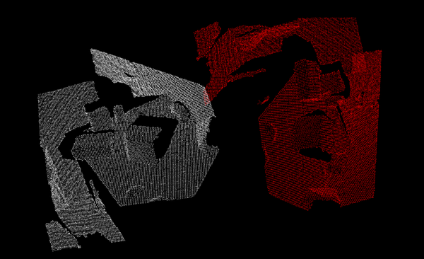
Clouds can be directly manipulated with transformations (translation, rotation, scaling). 3D transformations use a 4x4 matrix, which can be a little complicated to understand (specially when it comes to rotations), so check some book or tutorial before trying to use one. The transformed cloud will be saved to another object so you can keep both versions and use them as you wish.
#include <pcl/io/pcd_io.h>
#include <pcl/common/transforms.h>
#include <pcl/visualization/pcl_visualizer.h>

int
main(int argc, char** argv)
{
	// Objects for storing the point clouds.
	pcl::PointCloud<pcl::PointXYZ>::Ptr cloud(new pcl::PointCloud<pcl::PointXYZ>);
	pcl::PointCloud<pcl::PointXYZ>::Ptr transformed(new pcl::PointCloud<pcl::PointXYZ>);

	// Read a PCD file from disk.
	if (pcl::io::loadPCDFile<pcl::PointXYZ>(argv[1], *cloud) != 0)
	{
		return -1;
	}

	// Transformation matrix object, initialized to the identity matrix
	// (a null transformation).
	Eigen::Matrix4f transformation = Eigen::Matrix4f::Identity();

	// Set a rotation around the Z axis.
	float theta = M_PI / 2; // 180 degrees.
	transformation(0, 0) = cos(theta);
	transformation(0, 1) = -sin(theta);
	transformation(1, 0) = sin(theta);
	transformation(1, 1) = cos(theta);

	// Set a translation on the X axis.
	transformation(0, 3) = 1.0f; // 1 meter (positive direction).

	pcl::transformPointCloud(*cloud, *transformed, transformation);

	// Visualize both the original and the result.
	pcl::visualization::PCLVisualizer viewer(argv[1]);
	viewer.addPointCloud(cloud, "original");
	// The transformed one's points will be red in color.
	pcl::visualization::PointCloudColorHandlerCustom<pcl::PointXYZ> colorHandler(transformed, 255, 0, 0);
	viewer.addPointCloud(transformed, colorHandler, "transformed");
	// Add 3D colored axes to help see the transformation.
	viewer.addCoordinateSystem(1.0, 0);

	while (!viewer.wasStopped())
	{
		viewer.spinOnce();
	}
}
Using indices
Many of PCL's algorithms return indices. Indices are just a list of some of the points of a cloud (not the points themselves with all their data, but just their index in the cloud). For example, a cylinder segmentation algorithm will give you as output a list of points that were considered to fit the cylinder model. You can then use the indices to extract the points to a second cloud for further work with the "pcl::ExtractIndices" class. Its "setNegative()" function will instruct it to extract the points NOT indexed (so you can remove all cylinder-shaped clusters from the cloud).
#include <pcl/io/pcd_io.h>
#include <pcl/filters/extract_indices.h>
#include <pcl/segmentation/sac_segmentation.h>

#include <vector>

int
main(int argc, char** argv)
{
	// Objects for storing the point clouds.
	pcl::PointCloud<pcl::PointXYZ>::Ptr cloudAll(new pcl::PointCloud<pcl::PointXYZ>);
	pcl::PointCloud<pcl::PointXYZ>::Ptr cloudExtracted(new pcl::PointCloud<pcl::PointXYZ>);

	// Read a PCD file from disk.
	if (pcl::io::loadPCDFile<pcl::PointXYZ>(argv[1], *cloudAll) != 0)
	{
		return -1;
	}

	// Plane segmentation (do not worry, we will see this later).
	pcl::ModelCoefficients::Ptr coefficients(new pcl::ModelCoefficients);
	pcl::SACSegmentation<pcl::PointXYZ> segmentation;
	segmentation.setOptimizeCoefficients(true);
	segmentation.setModelType(pcl::SACMODEL_PLANE);
	segmentation.setMethodType(pcl::SAC_RANSAC);
	segmentation.setDistanceThreshold(0.01);
	segmentation.setInputCloud(cloudAll);

	// Object for storing the indices.
	pcl::PointIndices::Ptr pointIndices(new pcl::PointIndices);

	segmentation.segment(*pointIndices, *coefficients);

	// Object for extracting points from a list of indices.
	pcl::ExtractIndices<pcl::PointXYZ> extract;
	extract.setInputCloud(cloudAll);
	extract.setIndices(pointIndices);
	// We will extract the points that are NOT indexed (the ones that are not in a plane).
	extract.setNegative(true);
	extract.filter(*cloudExtracted);
}
- Input: Points, Indices, [Negative mode]
- Output: Points
- Tutorial: Extracting indices from a PointCloud
- API: pcl::PointIndices, pcl::ExtractIndices
- Download
Removing NaNs
The cloud retrieved from the sensor may contain several kind of measurement errors and/or inaccuracies. One of them is the presence of NaN (Not a Number) values in the coordinates of some points, as you can see in the following file:
# .PCD v0.7 - Point Cloud Data file format
VERSION 0.7
FIELDS x y z rgba
SIZE 4 4 4 4
TYPE F F F U
COUNT 1 1 1 1
WIDTH 640
HEIGHT 480
VIEWPOINT 0 0 0 1 0 0 0
POINTS 307200
DATA ascii
nan nan nan 10135463
nan nan nan 10398635
nan nan nan 10070692
nan nan nan 10268071
...
Cloud objects have a member function called "is_dense()" that will return true if all points have valid, finite values. A NaN indicates that there was a problem measuring the distance to that point, maybe because the sensor was too close or too far, or because the surface was reflective.
Sadly, many of PCL's algorithms will fail if even a single NaN is present in the cloud you feed them as input, with a message like "Assertion `point_representation_->isValid (point) && "Invalid (NaN, Inf) point coordinates given to radiusSearch!"' failed.". If this happens, you will have to remove such values from the cloud. You can use a program like the following to "clean" a cloud from all NaN points:
#include <pcl/io/pcd_io.h>
#include <pcl/filters/filter.h>

int
main(int argc, char** argv)
{
	if (argc != 3)
	{
		std::cout << "\tUsage: " << argv[0] << " <input cloud> <output cloud>" << std::endl;

		return -1;
	}

	// Object for storing the point cloud.
	pcl::PointCloud<pcl::PointXYZ>::Ptr cloud(new pcl::PointCloud<pcl::PointXYZ>);

	// Read a PCD file from disk.
	if (pcl::io::loadPCDFile<pcl::PointXYZ>(argv[1], *cloud) != 0)
	{
		return -1;
	}

	// The mapping tells you to what points of the old cloud the new ones correspond,
	// but we will not use it.
	std::vector<int> mapping;
	pcl::removeNaNFromPointCloud(*cloud, *cloud, mapping);

	// Save it back.
	pcl::io::savePCDFileASCII(argv[2], *cloud);
}
The problem with this method is that it will not keep the cloud organized. All clouds store a "width" and a "height" variable. In unorganized clouds, the total number of points is the same as the width, and the height is set to 1. In organized clouds (like the ones taken from camera-like sensors such as Kinect or Xtion), the width and the height are the same that the pixels of the image resolution the sensor works with. Points are distributed in rows like in the depth image, and every one of them corresponds to a pixel. The member function "isOrganized()" will return true if the height is greater than 1.
Because removing NaNs will change the number of points of the cloud, it can no longer be kept organized with the original width/height ratio, so the function will set the height to 1. This is not a big issue, as only a few of PCL's algorithms work explicitly with organized clouds (and they mostly use it for optimization), but you must take it into account.
- Input: Cloud
- Output: Cloud without NaNs
- API: pcl::removeNaNFromPointCloud()
- Download
Visualization
As you can see, it is possible to iterate through the cloud and print the information of each point to console, but this is cumbersome. Sometimes you just want to visualize the cloud to check something. PCL can create a window for you and display it, letting users pan and zoom their way around. The simplest method is the following one:
#include <pcl/io/pcd_io.h>
#include <pcl/visualization/cloud_viewer.h>

int
main(int argc, char** argv)
{
	// Object for storing the point cloud.
	pcl::PointCloud<pcl::PointXYZ>::Ptr cloud(new pcl::PointCloud<pcl::PointXYZ>);

	// Read a PCD file from disk.
	if (pcl::io::loadPCDFile<pcl::PointXYZ>(argv[1], *cloud) != 0)
	{
		return -1;
	}

	// Cloud viewer object. You can set the window title.
	pcl::visualization::CloudViewer viewer(argv[1]);
	viewer.showCloud(cloud);
	while (!viewer.wasStopped())
	{
		// Do nothing but wait.
	}
}
The program will remain active until you close the window with Alt+F4 or press Q. For a fully-featured visualizer class, check the second tutorial link below.
- Tutorials: The CloudViewer, PCLVisualizer
- API: pcl::visualization::CloudViewer
- Download
Feature estimation
A feature of a point is some characteristic that can help us to tell it apart from a different point. Of course, you could say that the XYZ coordinates would be characteristic enough, but when interpolating the data of two different, yet corresponding, clouds, they become useless. We need something better, that will have similar values when computed for the same spot of a surface in both sets.
Normals are an example of a very simple feature. 3D features will be important later in our tutorials, when we talk about descriptors (more detailed "signatures" of points used for close matching).
Normal estimation
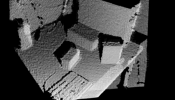
As you may remember from geometry class, the normal of a plane is an unit vector that is perpendicular to it. The normal of a surface at a point is defined as the vector that is perpendicular to the plane that is tangent to the surface at the point. Surface normals can be calculated for the points of a cloud, too. It is considered a feature, albeit not a very discriminative one.
I will not go into detail with the math of the estimation method, but you just have to know that is uses the nearest neighbors (the points that are closest to the one we are calculating the normal for) to find out the tangent plane and the normal vector. You can customize the method with the search radius (think about a sphere of that radius, centered in the point; all neighboring points that lie within will be used for the computation) and the viewpoint (by default, the output normals will be directionless; by supposing that all vectors must point towards the camera - because otherwise they would belong to surfaces that are not visible from the sensor - they can all be re-oriented accordingly).
Normals are also important because they give us information about the curvature of the surface at some point, which can be used to our advantage. Many of PCL's algorithms will require us to provide the normals of the input cloud. To estimate them, you can use the following code:
#include <pcl/io/pcd_io.h>
#include <pcl/features/normal_3d.h>
#include <boost/thread/thread.hpp>
#include <pcl/visualization/pcl_visualizer.h>

int
main(int argc, char** argv)
{
	// Object for storing the point cloud.
	pcl::PointCloud<pcl::PointXYZ>::Ptr cloud(new pcl::PointCloud<pcl::PointXYZ>);
	// Object for storing the normals.
	pcl::PointCloud<pcl::Normal>::Ptr normals(new pcl::PointCloud<pcl::Normal>);

	// Read a PCD file from disk.
	if (pcl::io::loadPCDFile<pcl::PointXYZ>(argv[1], *cloud) != 0)
	{
		return -1;
	}

	// Object for normal estimation.
	pcl::NormalEstimation<pcl::PointXYZ, pcl::Normal> normalEstimation;
	normalEstimation.setInputCloud(cloud);
	// For every point, use all neighbors in a radius of 3cm.
	normalEstimation.setRadiusSearch(0.03);
	// A kd-tree is a data structure that makes searches efficient. More about it later.
	// The normal estimation object will use it to find nearest neighbors.
	pcl::search::KdTree<pcl::PointXYZ>::Ptr kdtree(new pcl::search::KdTree<pcl::PointXYZ>);
	normalEstimation.setSearchMethod(kdtree);

	// Calculate the normals.
	normalEstimation.compute(*normals);

	// Visualize them.
	boost::shared_ptr<pcl::visualization::PCLVisualizer> viewer(new pcl::visualization::PCLVisualizer("Normals"));
	viewer->addPointCloud<pcl::PointXYZ>(cloud, "cloud");
	// Display one normal out of 20, as a line of length 3cm.
	viewer->addPointCloudNormals<pcl::PointXYZ, pcl::Normal>(cloud, normals, 20, 0.03, "normals");
	while (!viewer->wasStopped())
	{
		viewer->spinOnce(100);
		boost::this_thread::sleep(boost::posix_time::microseconds(100000));
	}
}
As you can see, normals are stored in "PointCloud" objects too, instantiated to the "Normal" type. If you ever extract some indices from a cloud before feeding them to an algorithm, be sure to do the same with the normals. I have not made use of the "setViewPoint()" function, but you get the idea.
Instead of "setRadiusSearch()", you can make use of "setKSearch()", which takes an integer, K. This will take into account a point's K nearest neighbors to compute the normal. Please mind that this can produce some odd results for points that are not in dense areas, as some of the "neighbors" will be too far from them.
- Input: Points, Search method, Radius | Neighbor count, [Indices], [Viewpoint]
- Output: Normals
- Tutorial: Estimating Surface Normals in a Point Cloud
- API: pcl::NormalEstimation
- Download
Decomposition
When I talk about decomposition, I mean the process of creating an ordered, organized data structure from the points of the cloud, with some purpose in mind like making further analysis easier, or performing filters.
k-d tree
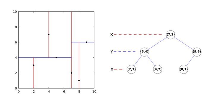
A k-d tree (k-dimensional tree) is a data structure that organizes a set of points in a k-dimensional space, in a way that makes range search operations very efficient (for example, finding the nearest neighbor of a point, which is the point that is closest to it in space; or finding all neighbors within a radius).
It is a binary tree, that is, every non-leaf node in it has two children nodes, the "left" and "right" ones. Each level splits space on a specific dimension. For example, in 3-dimensional space, at the root node (first level) all children would be split based on the first dimension, X (points having coordinates with greater X values would go to the right subtree, points with lesser values to the left one). At the second level (the nodes we just created), the split would be done on the Y axis, following the same criteria. At the third level (the grandchildren), we would use the Z axis. At the fourth level, we would get back to the X axis, and so on. Usually, the median point is chosen to be root at every level.
In PCL, creating a k-d tree from a cloud is a straightforward and fast operation:
Searching
The following code snippet shows you how to use a k-d tree to perform efficient searches:
#include <pcl/io/pcd_io.h>
#include <pcl/search/kdtree.h>

#include <iostream>
#include <vector>

int
main(int argc, char** argv)
{
	// Object for storing the point cloud.
	pcl::PointCloud<pcl::PointXYZ>::Ptr cloud(new pcl::PointCloud<pcl::PointXYZ>);

	// Read a PCD file from disk.
	if (pcl::io::loadPCDFile<pcl::PointXYZ>(argv[1], *cloud) != 0)
	{
		return -1;
	}

	// kd-tree object.
	pcl::search::KdTree<pcl::PointXYZ> kdtree;
	kdtree.setInputCloud(cloud);

	// We will find the 5 nearest neighbors of this point
	// (it does not have to be one of the cloud's, we can use any coordinate).
	pcl::PointXYZ point;
	point.x = 0.0524343;
	point.y = -0.58016;
	point.z = 1.776;
	// This vector will store the output neighbors.
	std::vector<int> pointIndices(5);
	// This vector will store their squared distances to the search point.
	std::vector<float> squaredDistances(5);
	// Perform the search, and print out results.
	if (kdtree.nearestKSearch(point, 5, pointIndices, squaredDistances) > 0)
	{
		std::cout << "5 nearest neighbors of the point:" << std::endl;
		for (size_t i = 0; i < pointIndices.size(); ++i)
			std::cout << "\t" << cloud->points[pointIndices[i]].x
					  << " " << cloud->points[pointIndices[i]].y
					  << " " << cloud->points[pointIndices[i]].z
					  << " (squared distance: " << squaredDistances[i] << ")" << std::endl;
	}

	// Now we find all neighbors within 3cm of the point
	// (inside a sphere of radius 3cm centered at the point).
	if (kdtree.radiusSearch(point, 0.03, pointIndices, squaredDistances) > 0)
	{
		std::cout << "Neighbors within 3cm:" << std::endl;
		for (size_t i = 0; i < pointIndices.size(); ++i)
			std::cout << "\t" << cloud->points[pointIndices[i]].x
					  << " " << cloud->points[pointIndices[i]].y
					  << " " << cloud->points[pointIndices[i]].z
					  << " (squared distance: " << squaredDistances[i] << ")" << std::endl;
	}
}
Another alternative would be "KdTreeFLANN", which makes use of FLANN (Fast Library for Approximate Nearest Neighbors).
- Input: Points, Radius | Neighbor count
- Output: Point indices, Squared distances
- Tutorial: How to use a KdTree to search
- API: pcl::search::KdTree, pcl::KdTreeFLANN
- Download
Octree
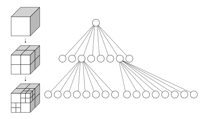
Like the k-d tree, the octree is an hierarchical tree data structure useful for searches, but also compression or downsampling. Each octree node (called a voxel, a term that will sound familiar for users of 3D engines, and which could be described as a "3D pixel", that is, a cube) has either eight children or no children. The root node describes a cubic bounding box which encapsulates all points. At every level, it becomes subdivided by a factor of 2 which results in an increased voxel resolution. That way, we can selectively give more resolution to certain zones.
Searching
Downsampling will be covered in a different section, so now I will show you how to perform searches with an octree:
#include <pcl/io/pcd_io.h>
#include <pcl/octree/octree.h>

#include <iostream>
#include <vector>

int
main(int argc, char** argv)
{
	// Object for storing the point cloud.
	pcl::PointCloud<pcl::PointXYZ>::Ptr cloud(new pcl::PointCloud<pcl::PointXYZ>);

	// Read a PCD file from disk.
	if (pcl::io::loadPCDFile<pcl::PointXYZ>(argv[1], *cloud) != 0)
	{
		return -1;
	}

	// Octree object, with a maximum resolution of 128
	// (resolution at lowest octree level).
	pcl::octree::OctreePointCloudSearch<pcl::PointXYZ> octree(128);
	octree.setInputCloud(cloud);
	octree.addPointsFromInputCloud();

	// We will find all neighbors within the same voxel as this point.
	// (it does not have to be one of the cloud's, we can use any coordinate).
	pcl::PointXYZ point;
	point.x = 0.0524343;
	point.y = -0.58016;
	point.z = 1.776;
	// This vector will store the output neighbors.
	std::vector<int> pointIndices;
	// Perform the search, and print out results.
	if (! octree.voxelSearch(point, pointIndices) > 0)
	{
		std::cout << "Neighbors in the same voxel:" << std::endl;
		for (size_t i = 0; i < pointIndices.size(); ++i)
			std::cout << "\t" << cloud->points[pointIndices[i]].x
					  << " " << cloud->points[pointIndices[i]].y
					  << " " << cloud->points[pointIndices[i]].z << std::endl;
	}

	// We will find the 5 nearest neighbors of the point.
	// This vector will store their squared distances to the search point.
	std::vector<float> squaredDistances;
	if (octree.nearestKSearch(point, 5, pointIndices, squaredDistances) > 0)
	{
		std::cout << "5 nearest neighbors of the point:" << std::endl;
		for (size_t i = 0; i < pointIndices.size(); ++i)
			std::cout << "\t" << cloud->points[pointIndices[i]].x
					  << " " << cloud->points[pointIndices[i]].y
					  << " " << cloud->points[pointIndices[i]].z
					  << " (squared distance: " << squaredDistances[i] << ")" << std::endl;
	}

	// Now we find all neighbors within 3cm of the point
	// (inside a sphere of radius 3cm centered at the point).
	// The point DOES have to belong in the cloud.
	if (octree.radiusSearch(point, 0.03, pointIndices, squaredDistances) > 0)
	{
		std::cout << "Neighbors within 3cm:" << std::endl;
		for (size_t i = 0; i < pointIndices.size(); ++i)
			std::cout << "\t" << cloud->points[pointIndices[i]].x
					  << " " << cloud->points[pointIndices[i]].y
					  << " " << cloud->points[pointIndices[i]].z
					  << " (squared distance: " << squaredDistances[i] << ")" << std::endl;
	}
}
As you can see, the code is mostly interchangeable with the one of the kd-tree.
- Input: Points, Radius | Neighbor count
- Output: Point indices, Squared distances
- Tutorial: Spatial Partitioning and Search Operations with Octrees
- API: pcl::search::Octree, pcl::octree::OctreePointCloudSearch
- Download
Compressing/Decompressing
On the other hand, this is the code needed to compress and decompress a point cloud with PCL:
#include <pcl/io/pcd_io.h>
#include <pcl/compression/octree_pointcloud_compression.h>
#include <boost/thread/thread.hpp>
#include <pcl/visualization/pcl_visualizer.h>

int
main(int argc, char** argv)
{
	// Objects for storing the point clouds.
	pcl::PointCloud<pcl::PointXYZ>::Ptr cloud(new pcl::PointCloud<pcl::PointXYZ>);
	pcl::PointCloud<pcl::PointXYZ>::Ptr decompressedCloud(new pcl::PointCloud<pcl::PointXYZ>);

	// Read a PCD file from disk.
	if (pcl::io::loadPCDFile<pcl::PointXYZ>(argv[1], *cloud) != 0)
	{
		return -1;
	}

	// Octree compressor object.
	// Check /usr/include/pcl-<version>/pcl/compression/compression_profiles.h for more profiles.
	// The second parameter enables the output of information.
	pcl::io::OctreePointCloudCompression<pcl::PointXYZ> octreeCompression(pcl::io::MED_RES_ONLINE_COMPRESSION_WITHOUT_COLOR, true);
	// Stringstream that will hold the compressed cloud.
	std::stringstream compressedData;

	// Compress the cloud (you would save the stream to disk).
	octreeCompression.encodePointCloud(cloud, compressedData);

	// Decompress the cloud.
	octreeCompression.decodePointCloud(compressedData, decompressedCloud);

	// Display the decompressed cloud.
	boost::shared_ptr<pcl::visualization::PCLVisualizer> viewer(new pcl::visualization::PCLVisualizer("Octree compression"));
	viewer->addPointCloud<pcl::PointXYZ>(decompressedCloud, "cloud");
	while (!viewer->wasStopped())
	{
		viewer->spinOnce(100);
		boost::this_thread::sleep(boost::posix_time::microseconds(100000));
	}
}
As you can see, the process has decreased the amount of points in the cloud. The default parameters of the "OctreePointCloudCompression" object establish an octree resolution (at lowest level) of 1cm, and a coordinate precision of 1mm. These values can of course be changed to suit your needs, but simplifying the cloud in this way is an useful operation that we will cover later.
- Input: Points, Resolution, Compression profile
- Output: Compressed stream
- Tutorial: Point Cloud Compression
- API: pcl::io::OctreePointCloudCompression
- Download
Detecting changes
PCL has an octree-based object that allows to detect changes between two point clouds (for example, two clouds taken one after another with an OpenNI device). This object stores the trees of both clouds at the same time, and compares them, returning a list of indices of the points that are new in the second cloud (they did not exist in the first):
#include <pcl/io/pcd_io.h>
#include <pcl/octree/octree.h>

#include <iostream>

int
main(int argc, char** argv)
{
	// Objects for storing the point clouds.
	pcl::PointCloud<pcl::PointXYZ>::Ptr cloudA(new pcl::PointCloud<pcl::PointXYZ>);
	pcl::PointCloud<pcl::PointXYZ>::Ptr cloudB(new pcl::PointCloud<pcl::PointXYZ>);

	// Read two PCD files from disk.
	if (pcl::io::loadPCDFile<pcl::PointXYZ>(argv[1], *cloudA) != 0)
	{
		return -1;
	}
	if (pcl::io::loadPCDFile<pcl::PointXYZ>(argv[2], *cloudB) != 0)
	{
		return -1;
	}

	// Change detector object, with a resolution of 128
	// (resolution at lowest octree level).
	pcl::octree::OctreePointCloudChangeDetector<pcl::PointXYZ> octree(128.0f);

	// Add cloudA to the octree.
	octree.setInputCloud(cloudA);
	octree.addPointsFromInputCloud();
	// The change detector object is able to store two clouds at the same time;
	// with this we can reset the buffer but keep the previous tree saved.
	octree.switchBuffers();
	// Now, add cloudB to the octree like we did before.
	octree.setInputCloud(cloudB);
	octree.addPointsFromInputCloud();

	std::vector<int> newPoints;
	// Get a vector with the indices of all points that are new in cloud B,
	// when compared with the ones that existed in cloud A.
	octree.getPointIndicesFromNewVoxels(newPoints);
	for (size_t i = 0; i < newPoints.size(); ++i)
	{
		std::cout << "Point (" << cloudB->points[newPoints[i]].x << ", "
				  << cloudB->points[newPoints[i]].y << ", "
				  << cloudB->points[newPoints[i]].z
				  << ") was not in cloud A but is in cloud B" << std::endl;
	}
	std::cout << newPoints.size() << std::endl;
}
- Input: First cloud, Second cloud, Resolution
- Output: Point indices
- Tutorial: Spatial change detection on unorganized point cloud data
- API: pcl::octree::OctreePointCloudChangeDetector
- Download
Filtering
The raw point cloud, as returned from the sensor, usually needs some kind of polishing before being handed to processing algorithms. Normally, this is due to the low precision of the sensor, which leads to noise, incorrect measurements, holes in surfaces... Sometimes it is just the opposite: the cloud has so many points that processing it would take forever. Luckily, several filtering methods exist to "fix" many recurring errors in point clouds.
Passthrough filter
A passthrough filter will remove any point from the cloud whose values do not fall in a certain range, user-given. For example, if you wanted to discard all points farther away than, say, 3 meters, you would run the filter on the Z coordinate with a range of [0,3]. This filter can be useful to discard unneeded objects from the cloud, but you may have to adapt a different reference frame if the default one (relative to the sensor) is not fitting. For example, filtering on the Y value to remove all points not sitting on a table will yield unwanted results of the camera was at an odd angle.
#include <pcl/io/pcd_io.h>
#include <pcl/filters/passthrough.h>

int
main(int argc, char** argv)
{
	// Objects for storing the point clouds.
	pcl::PointCloud<pcl::PointXYZ>::Ptr cloud(new pcl::PointCloud<pcl::PointXYZ>);
	pcl::PointCloud<pcl::PointXYZ>::Ptr filteredCloud(new pcl::PointCloud<pcl::PointXYZ>);

	// Read a PCD file from disk.
	if (pcl::io::loadPCDFile<pcl::PointXYZ>(argv[1], *cloud) != 0)
	{
		return -1;
	}

	// Filter object.
	pcl::PassThrough<pcl::PointXYZ> filter;
	filter.setInputCloud(cloud);
	// Filter out all points with Z values not in the [0-2] range.
	filter.setFilterFieldName("z");
	filter.setFilterLimits(0.0, 2.0);

	filter.filter(*filteredCloud);
}
The "setFilterLimitsNegative()" function (not seen in the example) will tell the filter object whether to return the points inside the range ("false", the default value) or outside it ("true").
- Input: Points, Filter field, Filter limits, [Negative mode]
- Output: Filtered points
- Tutorial: Filtering a PointCloud using a PassThrough filter
- API: pcl::PassThrough
- Download
Conditional removal
Another way of getting the exact same result than with the previous example would be to use a conditional removal filter. We can build any kind of condition we want for the values of the point:
#include <pcl/io/pcd_io.h>
#include <pcl/filters/conditional_removal.h>

int
main(int argc, char** argv)
{
	// Objects for storing the point clouds.
	pcl::PointCloud<pcl::PointXYZ>::Ptr cloud(new pcl::PointCloud<pcl::PointXYZ>);
	pcl::PointCloud<pcl::PointXYZ>::Ptr filteredCloud(new pcl::PointCloud<pcl::PointXYZ>);

	// Read a PCD file from disk.
	if (pcl::io::loadPCDFile<pcl::PointXYZ>(argv[1], *cloud) != 0)
	{
		return -1;
	}

	// We must build a condition.
	// And "And" condition requires all tests to check true. "Or" conditions also available.
	pcl::ConditionAnd<pcl::PointXYZ>::Ptr condition(new pcl::ConditionAnd<pcl::PointXYZ>);
	// First test, the point's Z value must be greater than (GT) 0.
	condition->addComparison(pcl::FieldComparison<pcl::PointXYZ>::ConstPtr(new pcl::FieldComparison<pcl::PointXYZ>("z", pcl::ComparisonOps::GT, 0.0)));
	// Second test, the point's Z value must be less than (LT) 2.
	condition->addComparison(pcl::FieldComparison<pcl::PointXYZ>::ConstPtr(new pcl::FieldComparison<pcl::PointXYZ>("z", pcl::ComparisonOps::LT, 2.0)));
	// Checks available: GT, GE, LT, LE, EQ.

	// Filter object.
	pcl::ConditionalRemoval<pcl::PointXYZ> filter(condition);
	filter.setInputCloud(cloud);
	// If true, points that do not pass the filter will be set to a certain value (default NaN).
	// If false, they will be just removed, but that could break the structure of the cloud
	// (organized clouds are clouds taken from camera-like sensors that return a matrix-like image).
	filter.setKeepOrganized(true);
	// If keep organized was set true, points that failed the test will have their Z value set to this.
	filter.setUserFilterValue(0.0);

	filter.filter(*filteredCloud);
}
- Input: Points, Condition, [Keep organized]
- Output: Filtered points
- Tutorial: Removing outliers using a Conditional or RadiusOutlier removal
- API: pcl::ConditionalRemoval
- Download
Outlier removal
Outliers are lonely points that are spread here and there in the cloud, like annoying mosquitoes. They are the product of the sensor's inaccuracy, which registers measurements where there should not be any. Outliers are considered undesired noise because they can introduce errors in calculations, like for example the normal estimation. Hence, trimming they out of the cloud will not only make computations faster (because the less points there are, the less time it takes, as we will see with downsampling) but also help us get more precise values.
Radius-based
The radius-based outlier removal is the simplest method of all. You must specify a search radius and the minimum number of neighbors than a point must have to avoid being labelled as outlier. The algorithm will then iterate through all points (which can be slow in if the cloud is big) and perform the check: if less than that number of points are found within the radius, it is removed.
#include <pcl/io/pcd_io.h>
#include <pcl/filters/radius_outlier_removal.h>

int
main(int argc, char** argv)
{
	// Objects for storing the point clouds.
	pcl::PointCloud<pcl::PointXYZ>::Ptr cloud(new pcl::PointCloud<pcl::PointXYZ>);
	pcl::PointCloud<pcl::PointXYZ>::Ptr filteredCloud(new pcl::PointCloud<pcl::PointXYZ>);

	// Read a PCD file from disk.
	if (pcl::io::loadPCDFile<pcl::PointXYZ>(argv[1], *cloud) != 0)
	{
		return -1;
	}

	// Filter object.
	pcl::RadiusOutlierRemoval<pcl::PointXYZ> filter;
	filter.setInputCloud(cloud);
	// Every point must have 10 neighbors within 15cm, or it will be removed.
	filter.setRadiusSearch(0.15);
	filter.setMinNeighborsInRadius(10);

	filter.filter(*filteredCloud);
}
All PCL classes that inherit from "pcl::FilterIndices" (like "pcl::RadiusOutlierRemoval") provide the function "setNegative()", which if set to true, makes the filter return the points that did NOT pass the filter.
- Input: Points, Radius, Neighbor count
- Output: Filtered points
- Tutorial: Removing outliers using a Conditional or RadiusOutlier removal
- API: pcl::RadiusOutlierRemoval
- Download
Statistical
The statistical outlier removal process is a bit more refined. First, for every point, the mean distance to its K neighbors is computed. Then, if we asume that the result is a normal (gaussian) distribution with a mean μ and a standard deviation σ, we can deem it safe to remove all points with mean distances that fall out of the global mean plus deviation. Basically, it runs a statistical analysis of the distances between neighboring points, and trims all which are not considered "normal" (you define what "normal" is with the parameters of the algorithm).
#include <pcl/io/pcd_io.h>
#include <pcl/filters/statistical_outlier_removal.h>

int
main(int argc, char** argv)
{
	// Objects for storing the point clouds.
	pcl::PointCloud<pcl::PointXYZ>::Ptr cloud(new pcl::PointCloud<pcl::PointXYZ>);
	pcl::PointCloud<pcl::PointXYZ>::Ptr filteredCloud(new pcl::PointCloud<pcl::PointXYZ>);

	// Read a PCD file from disk.
	if (pcl::io::loadPCDFile<pcl::PointXYZ>(argv[1], *cloud) != 0)
	{
		return -1;
	}

	// Filter object.
	pcl::StatisticalOutlierRemoval<pcl::PointXYZ> filter;
	filter.setInputCloud(cloud);
	// Set number of neighbors to consider to 50.
	filter.setMeanK(50);
	// Set standard deviation multiplier to 1.
	// Points with a distance larger than 1 standard deviation of the mean distance will be outliers.
	filter.setStddevMulThresh(1.0);

	filter.filter(*filteredCloud);
}
You can make use of "setNegative()" with this filter too.
- Input: Points, Neighbor count, Deviation multiplier
- Output: Filtered points
- Tutorial: Removing outliers using a StatisticalOutlierRemoval filter
- API: pcl::StatisticalOutlierRemoval
- Download
Resampling
Resampling means changing the number of points of the cloud, either by reducing (downsampling) or increasing (upsampling). Both have a purpose, as we will see.
Downsampling
A sensor like Kinect or Xtion produces a cloud with 307200 (640x480) points. Believe it or not, that is a lot of information, and the new Kinect is already out there, working at a higher resolution. Keep in mind that, if we were to perform a simple operation on every point of a cloud, it would be of O(n), n being the number of points. If we had to compare every point with its k nearest neighbors, it would be O(nk). You may have noticed by now that some of the algorithms I showed you take several seconds to run on your PC; you now know why.
Optimization techniques are being implemented as I write this to allow PCL to employ the computer's GPU (graphic card) to perform the computations using CUDA. Many classes already provide an alternative in the "pcl::gpu" namespace. This offers dramatic improvements in speed, but it is not always a possibility.
Another option is to reduce the complexity of the cloud, that is, to remove all points that are not needed for the purpose. There are several ways to do this. You could trim all outliers from the cloud, then perform segmentation to extract only the parts that interest you. A common operation is also downsampling, which will give you back a cloud that, for all intents and purposes, equivalent to the original one, despite having less points.
Downsampling is done via voxelization. I already explained what voxels were in the octree section. The cloud is divided in multiple cube-shaped regions with the desired resolution. Then, all points inside every voxel are processed so only one remains. The simplest way would be to randomly select one of them, but a more accurate approach would be to compute the centroid, which is the point whose coordinates are the mean values of all the points that belong to the voxel.
If done with sensible parameters, downsampling will yield results that are precise enough to work with, at the cost of less CPU power.
#include <pcl/io/pcd_io.h>
#include <pcl/filters/voxel_grid.h>

int
main(int argc, char** argv)
{
	// Objects for storing the point clouds.
	pcl::PointCloud<pcl::PointXYZ>::Ptr cloud(new pcl::PointCloud<pcl::PointXYZ>);
	pcl::PointCloud<pcl::PointXYZ>::Ptr filteredCloud(new pcl::PointCloud<pcl::PointXYZ>);

	// Read a PCD file from disk.
	if (pcl::io::loadPCDFile<pcl::PointXYZ>(argv[1], *cloud) != 0)
	{
		return -1;
	}

	// Filter object.
	pcl::VoxelGrid<pcl::PointXYZ> filter;
	filter.setInputCloud(cloud);
	// We set the size of every voxel to be 1x1x1cm
	// (only one point per every cubic centimeter will survive).
	filter.setLeafSize(0.01f, 0.01f, 0.01f);

	filter.filter(*filteredCloud);
}
As an alternative, take a look at the class pcl::UniformSampling, which does essentially the same.
- Input: Points, Voxel size
- Output: Downsampled cloud
- Tutorial: Downsampling a PointCloud using a VoxelGrid filter
- API: pcl::VoxelGrid
- Download
Reconstruction
Surface smoothing
As stated, depth sensors are not very accurate, and the resulting clouds have measurement errors, outliers, holes in surfaces, etc. Surfaces can be reconstructed by means of an algorithm, that iterates through all points and interpolates the data, trying to guess how the original surface was. PCL uses the Moving Least Squares (MLS) algorithm for this. Performing this step is important, because the resulting cloud's normals will be more accurate.
Surface smoothing is easily done with the following code:
#include <pcl/io/pcd_io.h>
#include <pcl/surface/mls.h>

int
main(int argc, char** argv)
{
	// Objects for storing the point clouds.
	pcl::PointCloud<pcl::PointXYZ>::Ptr cloud(new pcl::PointCloud<pcl::PointXYZ>);
	// The output will also contain the normals.
	pcl::PointCloud<pcl::PointNormal>::Ptr smoothedCloud(new pcl::PointCloud<pcl::PointNormal>);

	// Read a PCD file from disk.
	if (pcl::io::loadPCDFile<pcl::PointXYZ>(argv[1], *cloud) != 0)
	{
		return -1;
	}

	// Smoothing object (we choose what point types we want as output).
	pcl::MovingLeastSquares<pcl::PointXYZ, pcl::PointNormal> filter;
	filter.setInputCloud(cloud);
	// Use all neighbors in a radius of 3cm.
	filter.setSearchRadius(0.03);
	// If true, the surface and normal are approximated using a polynomial estimation
	// (if false, only a tangent one).
	filter.setPolynomialFit(true);
	// We can tell the algorithm to also compute smoothed normals (optional).
	filter.setComputeNormals(true);
	// kd-tree object for performing searches.
	pcl::search::KdTree<pcl::PointXYZ>::Ptr kdtree;
	filter.setSearchMethod(kdtree);

	filter.process(*smoothedCloud);
}
- Input: Points, Search radius, [Polynomial fit], [Compute normals]
- Output: Smoothed cloud
- Tutorial: Smoothing and normal estimation based on polynomial reconstruction
- API: pcl::MovingLeastSquares
- Download
Go to root: PhD-3D-Object-Tracking
Links to articles:
PCL/OpenNI tutorial 0: The very basics
PCL/OpenNI tutorial 1: Installing and testing
PCL/OpenNI tutorial 2: Cloud processing (basic)
PCL/OpenNI tutorial 3: Cloud processing (advanced)
PCL/OpenNI tutorial 4: 3D object recognition (descriptors)
